Differentiable Stellarator Optimization

Purpose

GKX’s public optimization examples are actual VMEC-JAX QA stellarator workflows with GKX transport objectives appended to the VMEC-JAX objective tuple list.

• The paper-facing VMEC-JAX path starts from the upstream fixed-boundary QA script examples/optimization/QA_optimization.py and keeps its solved- equilibrium objective structure: aspect ratio, high-weight mean iota, and quasisymmetry. GKX transport enters as one additional objective tuple.

• Reduced max-mode-1 synthetic controls are development diagnostics only. They live outside examples/optimization and are not README-facing stellarator-optimization examples.

The VMEC-JAX-style scripts preserve the current upstream QA constants: mode-1-through-5 continuation, ASPECT_TARGET = 6.0, IOTA_TARGET = 0.42, and a weight of 10 on the mean-iota residual. The GKX objective is appended with a small editable weight so the QA/aspect/iota gates remain dominant. Any production nonlinear heat-flux claim still requires matched long post-transient GKX audits, replicate statistics, and running-average convergence checks.

Source Map

• Core API: gkx.objectives.stellarator

• Current VMEC-JAX equilibrium-to-flux-tube adapter: vmex.core.turbulence.flux_tube_geometry

• Current growth, quasilinear, and reduced nonlinear-window callbacks: vmex.core.turbulence.turbulent_growth_rate, quasilinear_flux_proxy, and nonlinear_heat_flux_proxy

• Lower-level GKX objective kernels used by those callbacks: gkx.solver_linear_operator_matrix_from_geometry(), gkx.solver_objective_vector_from_geometry()

• Production in-memory geometry boundary: gkx.flux_tube_geometry_from_vmec_boozer_state()

• Production-adjacent linear/quasilinear objective evaluator: gkx.vmec_boozer_solver_objective_vector_from_state()

• Scalar optimizer hook: gkx.vmec_boozer_scalar_objective_from_state()

• Multi-point objective table and aggregate hooks: gkx.vmec_boozer_solver_objective_table_from_state(), gkx.vmec_boozer_aggregate_scalar_objective_from_state()

• VMEC-state finite-difference sensitivity audit: gkx.vmec_boozer_scalar_objective_finite_difference_report()

• Multi-point finite-difference sensitivity audit: gkx.vmec_boozer_aggregate_scalar_objective_finite_difference_report()

• Fast branch-continuity and sensitivity gate: gkx.solver_objective_branch_gradient_report()

• VMEC-JAX-style growth-rate script: QA_optimization_linear_ITG.py

• VMEC-JAX-style quasilinear-flux script: QA_optimization_quasilinear_ITG.py

• VMEC-JAX-style nonlinear-window script: QA_optimization_nonlinear_ITG.py

• Optimization examples README: README.md

VMEC-JAX-Style QA Transport Scripts

The three solved-boundary examples follow the current upstream vmex/examples/optimization/QA_optimization.py protocol. They use VmecInput, solve_equilibrium, and opt.least_squares directly; no legacy fixed-boundary optimizer object, objective-term wrapper, or disk bridge is involved:

python examples/optimization/QA_optimization_linear_ITG.py
python examples/optimization/QA_optimization_quasilinear_ITG.py
python examples/optimization/QA_optimization_nonlinear_ITG.py

The circular seed perturbation, mode-1-through-5 continuation, QA residual, aspect target A=6, and mean-iota target 0.42 match upstream. GKX adds only the last tuple:

objective_terms = [
    (qs, 0.0, 1.0),
    (opt.aspect_ratio, ASPECT_TARGET, 1.0),
    (opt.mean_iota, IOTA_TARGET, 10.0),
    (transport_objective, 0.0, TRANSPORT_WEIGHT),
]
result = opt.least_squares(
    objective_terms,
    inp,
    max_mode=max_mode,
    jac=JAC,
    use_ess=True,
)

transport_objective(state, runtime) calls one of the current VMEC-JAX GKX adapters on a fixed ITG flux tube:

• turbulent_growth_rate returns the dominant linear growth rate. It is traceable through geometry and the eigensolve, so JAC="implicit" composes the equilibrium implicit Jacobian with the turbulence derivative.

• quasilinear_flux_proxy returns the eigenvector-weighted mixing-length diagnostic. It sets JAC=None because current JAX does not differentiate nonsymmetric eigenvectors in the required mode.

• nonlinear_heat_flux_proxy applies the documented smooth saturation rule to the same linear mode. It also sets JAC=None and remains a candidate- generation proxy, not a nonlinear time average.

This derivative policy is deliberate: unsupported eigenvector derivatives are not replaced by a zero or mislabeled as end-to-end AD. Each example exposes the surface index, field-line label, angular and velocity-space resolution, selected k_y index, and density/temperature gradients as top-level constants.

The optimizer output must then pass solved-equilibrium geometry gates and the separate long-window transport workflow.

Only converged, replicated, post-transient nonlinear windows can support a nonlinear turbulent-flux reduction. Linear growth, quasilinear screening, and reduced nonlinear-window residuals retain their narrower claim scopes.

Optimizer Strategy and Literature Anchor

The optimizer choice depends on the observable being optimized:

• Constraints-only QA baseline. Use the upstream VMEC-JAX/SIMSOPT-style nonlinear least-squares structure for aspect ratio, mean iota, and quasisymmetry. This is the smoothest part of the workflow and is closest to the standard stellarator-optimization pattern used in SIMSOPT and its quasisymmetry examples. Bound-aware trust-region reflective least squares is also the relevant SciPy baseline because it is designed for nonlinear least-squares problems with bounds.

• Linear-growth and quasilinear objectives. Use the current VMEC-JAX least-squares owner with the implicit equilibrium Jacobian for growth and a finite-difference outer Jacobian for eigenvector-weighted quasilinear objectives. Require tangent/finite-difference gates on the selected sample set. A linear gyrokinetic or quasilinear proxy remains a proxy until nonlinear validation is complete.

• Long nonlinear heat flux. Do not treat the long-time post-transient heat flux as a smooth least-squares residual. The nonlinear turbulence optimization literature reports noisy heat-flux traces and noisy parameter landscapes; smooth optimizers can stagnate on local minima. The direct nonlinear stellarator-optimization study by Kim et al. therefore used SPSA, because it estimates a stochastic gradient with only two objective evaluations and can tolerate noisy heat-flux averages. CMA-ES or Bayesian optimization are reasonable outer-loop comparators for low-dimensional, expensive, rugged scans, but they must be judged by matched nonlinear audits, not by reduced startup-window residuals.

Practical GKX policy:

1. Use current VMEC-JAX least squares for the strict constraints-only QA baseline, and keep an independently replayed WOUT as the common starting point.

2. Compare derivative policies only within identical comparison_fingerprint groups. Different sample sets, moment resolution, or objective transforms are separate campaigns, not optimizer comparisons.

3. Use growth first, then explicit quasilinear rules, then nonlinear-window screening. These runs choose candidates; they do not prove turbulent-flux reduction.

4. Promote a candidate only after matched initial/final nonlinear GKX audits pass the strict long-window policy: staged horizons 700,1100,1500, accepted average over t=[1100,1500], seed/timestep replication, and follow-up grid/window convergence for both baseline and optimized states.

5. If a nonlinear objective landscape is jagged, incomplete, or has failed neighboring points, use it as an optimizer-noise diagnostic only. Do not use it to claim a reliable gradient or a robust minimum.

Current optimizer evidence

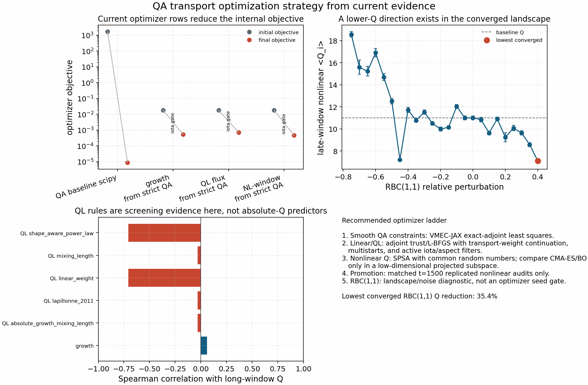
The strategy artifact below is regenerated from vmex_qa_full_sweep_panel.json and vmec_boundary_transport_landscape_rbc11_full.json. It encodes the present state of the optimizer lane:

• the strict max-mode-5 QA baseline is admitted;

• the linear-growth, quasilinear-flux, and nonlinear-window transport restarts reduce their internal objectives but remain diagnostic-only because the strict solved-WOUT gate is not met and the true matched t=1500 nonlinear audits fail the heat-flux-reduction promotion gate;

• the converged RBC(1,1) long-window landscape has a material lower-Q direction, with the lowest converged point near +40% reducing the post-transient <Q_i> by about 35% relative to the zero-offset baseline;

• the RBC(1,1) landscape is a noise/convergence diagnostic and must not be treated as an admission source or warm-start requirement for optimized QA stellarators;

• the current one-DOF landscape does not support an absolute-flux quasilinear promotion claim, so linear/QL metrics are used for screening and candidate generation until held-out nonlinear gates pass.

The report sidecars vmex_qa_optimizer_strategy_report.json and vmex_qa_optimizer_strategy_report.csv are the machine-readable claim boundary. In particular, nonlinear_absolute_optimization_promoted is intentionally false.

Broad nonlinear matrix outcome

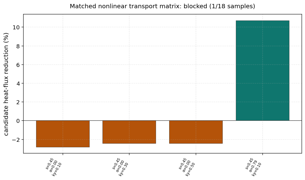
The strict broad nonlinear turbulent-flux optimization gate is intentionally separate from the scoped matched-audit examples above. It requires a completed 18-point matrix with three surfaces, two field-line labels, three k_y values, seed/timestep replication, and the post-transient averaging window t=[1100,1500]. The current max-mode-5 campaign did not pass this gate:

• accepted QA/ESS passed 9/18 samples and failed the required pass fraction;

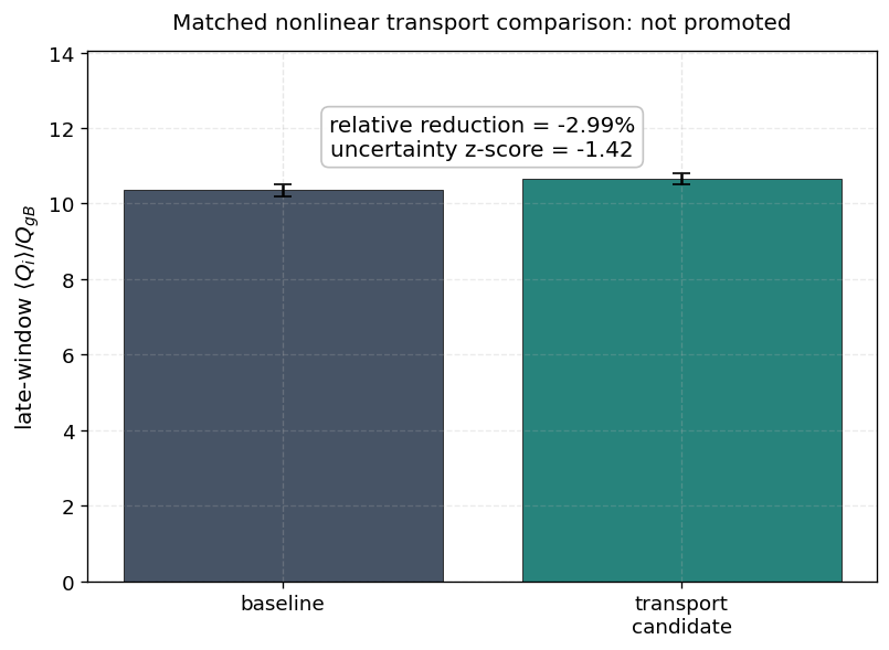
• projected weight 1e-3 failed early with only 1/18 passing samples and mean relative reduction below the 2% policy threshold;

• projected weight 5e-4 increased heat flux by about 2.99% on its first completed sample, so the family was stopped under the all-sample policy.

This is negative broad-promotion evidence, not a release failure for the scoped examples. It means the current release can cite reduced-objective plumbing and selected single-point matched audits, but it must not claim broad nonlinear turbulent-flux stellarator optimization. The machine-readable ledger is broad_nonlinear_transport_matrix_negative_evidence.json.

The early-stop logic is part of the scientific guardrail: under a required pass_fraction=1.0 policy, one failed sample is enough to prevent broad promotion. Stopping a failed family avoids spending GPU time on a candidate that cannot satisfy the documented gate.

Optimizer-Comparison Manifest

Optimizer comparisons should be launched from a single manifest, not from hand-edited shell history.

The tracked manifest sidecar vmex_qa_optimizer_comparison_manifest.json was generated with an older API generation and is retained as historical provenance. It records:

• one QA constraints baseline using current VMEC-JAX least squares;

• one matched command per transport observable from the common baseline: implicit equilibrium derivatives for growth and finite-difference outer Jacobians for quasilinear_flux and nonlinear_window_heat_flux;

• SPSA, CMA-ES, and Bayesian-optimization (bo) outer-loop contracts with deterministic metric-evaluation and nonlinear-audit command templates.

The manifest comparison fingerprint is part of the campaign contract. A method comparison is valid only when the sample set, Boozer resolution, moment resolution, objective transform, transport weight, optimizer budget, and strict nonlinear-audit policy match. The machine-readable landscape_policy keeps the RBC(1,1) scan diagnostic-only: it diagnoses objective roughness, metric disagreement, and required nonlinear averaging windows, but it does not admit optimized candidates or replace the VMEC-JAX simple-seed QA baseline. The campaign order is deterministic growth/QL screening first, SPSA for noisy long-window nonlinear Q, and CMA-ES or Bayesian optimization only as low-dimensional comparators. The derivative-free entries are reproducible outer-loop protocols, not VMEC-JAX optimizer methods. They become paper evidence only after their candidates pass the same matched long-window nonlinear gates as differentiable optimizer outputs.

The first office execution of this ladder is tracked as reduced-metric strategy evidence: vmex_qa_optimizer_ladder_resume_status.json and vmex_qa_optimizer_ladder_spsa_metric_summary.json. The scalar-trust and LBFGS-adjoint deterministic runs completed and passed the authoritative rerun-WOUT admission gate, but their solved-candidate gates remained false. The four SPSA plus/minus reduced nonlinear-window pairs also completed; the best reduced metrics are useful for optimizer-design triage, not for claiming a reduced long-window turbulent heat flux.

Key references for this policy are:

• Optimization of nonlinear turbulence in stellarators: direct nonlinear heat-flux optimization, SPSA for noisy heat-flux objectives, Boozer |B| panels, field-line/radius scans, and matched heat-flux traces.

• Direct Microstability Optimization of Stellarator Devices: linear gyrokinetic/quasilinear transport-proxy optimization balanced against quasisymmetry.

• SciPy least_squares: trust-region reflective least-squares reference behavior.

• JAXopt LBFGSB, Optax Adam, and CMA-ES: implementation references for gradient-based, adaptive first-order, and derivative-free noisy/rugged optimization comparators.

Each optimization script also writes long-window initial/final nonlinear ITG audit manifests after saving the VMEC-JAX result. They are not launched by default because the audits are multi-hour GPU jobs; set RUN_LONG_NONLINEAR_AUDIT_COMMANDS = True inside the script to launch them, build replicated initial/final ensemble gates, and write the initial-vs-final nonlinear Q(t) comparison plot, or launch the generated run_manifest.json commands explicitly on the target workstation. The generated manifests now use the strict staged nonlinear policy described above; older t=[350,700] manifests should be treated as historical diagnostics unless rerun through the current policy. The manifest separates restart-ladder segment commands from direct full-horizon commands and adds a runtime-output gate over the accepted window, so a final t=1500 segment run from t=0 cannot be mistaken for a true t=1500 nonlinear audit.

The first full-sweep matched QA audit under this strict policy has been harvested from the office workstation, but it is not admitted. All raw baseline, growth-optimized, quasilinear-optimized, and nonlinear-window- optimized runtime jobs completed, yet the produced traces end near t=400. Because the strict postprocess requested t=[1100,1500], every replicated ensemble has n_finite_means = 0 and every matched baseline-vs-candidate comparison is passed = false with no finite relative reduction. The diagnostic artifacts are retained as docs/_static/optimized_equilibrium_replicates/vmec_qa_full_sweep_* and docs/_static/qa_strict_baseline_to_*_strict_baseline.*. They are command and admission-policy evidence, not nonlinear holdouts or optimization successes. A true relaunch must either follow the staged 700 -> 1100 -> 1500 restart ladder or use the manifest direct_full_horizon_launch_commands.

The corrected true-full-horizon relaunch is now fully harvested for the strict QA baseline plus the growth-objective, quasilinear-objective, and nonlinear-window-objective candidates. All four rows pass the fail-closed runtime-output gate and replicated seed/timestep ensemble gate over t=[1100,1500]. The baseline has ensemble mean <Q_i> = 11.580, mean relative spread 0.0381, and combined SEM/mean 0.0195. The growth candidate has ensemble mean <Q_i> = 11.510, mean relative spread 0.0427, and combined SEM/mean 0.0124. The quasilinear candidate has ensemble mean <Q_i> = 11.636, mean relative spread 0.0234, and combined SEM/mean 0.0164. The nonlinear-window candidate has ensemble mean <Q_i> = 11.609, mean relative spread 0.0366, and combined SEM/mean 0.0177. These artifacts close the question of whether the candidate traces are real saturated long-window signals, but they do not promote the candidates as transport optimizations: the matched growth comparison gives only 0.60% relative reduction with uncertainty z = 0.26 against the 4% promotion gate, while the quasilinear and nonlinear-window comparisons are slightly worse than baseline (-0.49%, z = -0.19; -0.25%, z = -0.09).

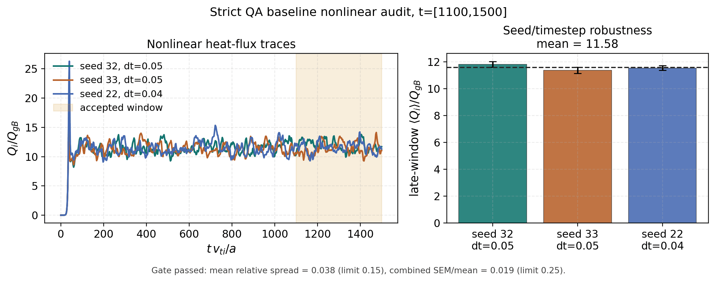
True full-horizon strict QA baseline audit. The late window t=[1100,1500] passes the seed/timestep robustness gate and provides the matched reference for the candidate comparisons below.

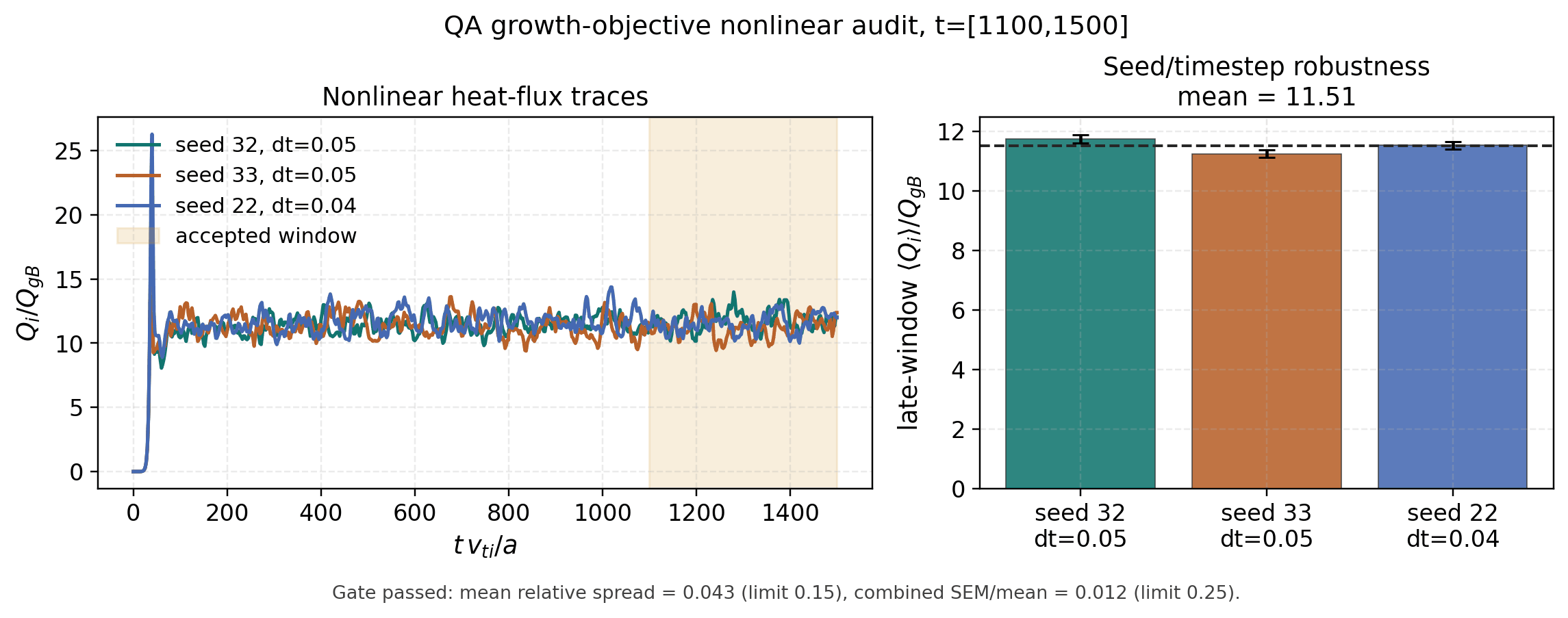
True full-horizon growth-objective QA audit. The late window t=[1100,1500] passes the seed/timestep robustness gate, but the panel is a candidate-audit artifact rather than a matched optimization-success claim.

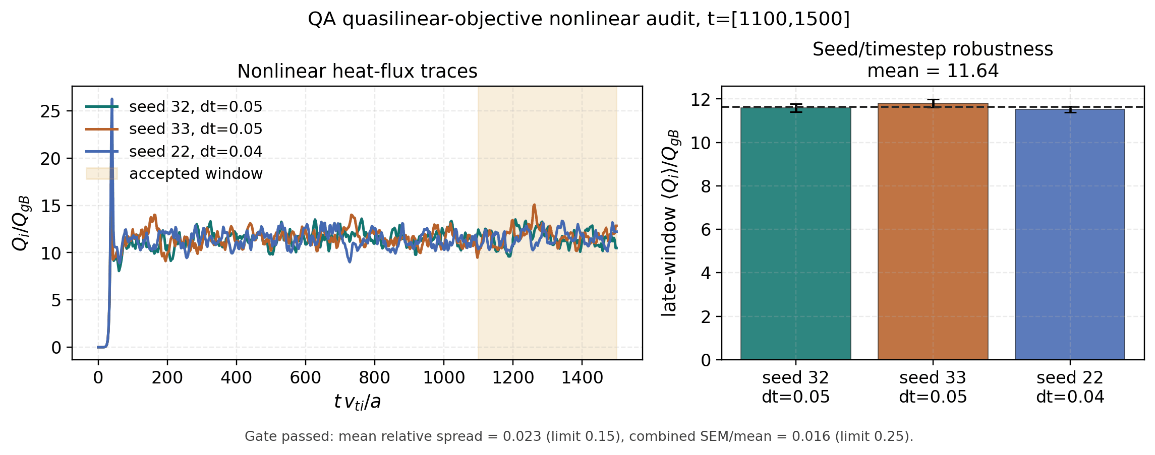
True full-horizon quasilinear-objective QA audit. The late-window ensemble passes the seed/timestep robustness gate, but its matched comparison below is slightly worse than the strict QA baseline.

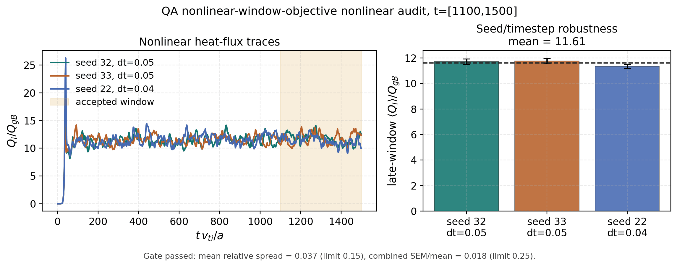
True full-horizon nonlinear-window-objective QA audit. The late-window ensemble is statistically robust across two seeds and one timestep variant; the matched baseline comparison below does not promote it as a reduction.

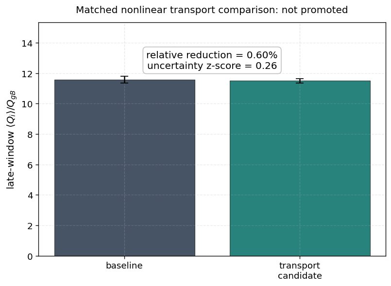
Matched baseline-to-growth nonlinear transport comparison. The growth objective produces only a 0.60% reduction with z = 0.26, so it does not pass the 4% promotion gate.

Matched baseline-to-quasilinear transport comparison. The quasilinear candidate is 0.49% higher than the strict QA baseline with z = -0.19, so it is not admitted as nonlinear transport reduction evidence.

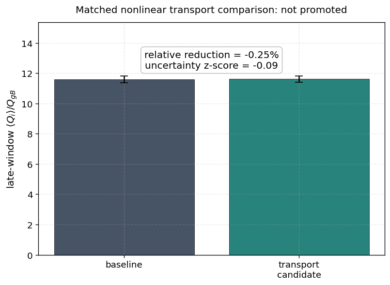
Matched baseline-to-nonlinear-window transport comparison. The candidate is slightly worse than the strict QA baseline in the long post-transient window and is not promoted.

README-facing strict QA optimizer sweep built from tracked VMEC-JAX WOUTs and GKX reduced transport residuals. The sidecar vmex_qa_full_sweep_panel.json records the exact artifact provenance.

Full Max-Mode-5 Optimizer Sweeps

For manuscript-facing comparisons between optimizer algorithms, run the full max_mode = 5 VMEC-JAX solved-boundary sweep on the workstation/GPU node and then build the comparison panel from the real history.json and wout_final.nc outputs.

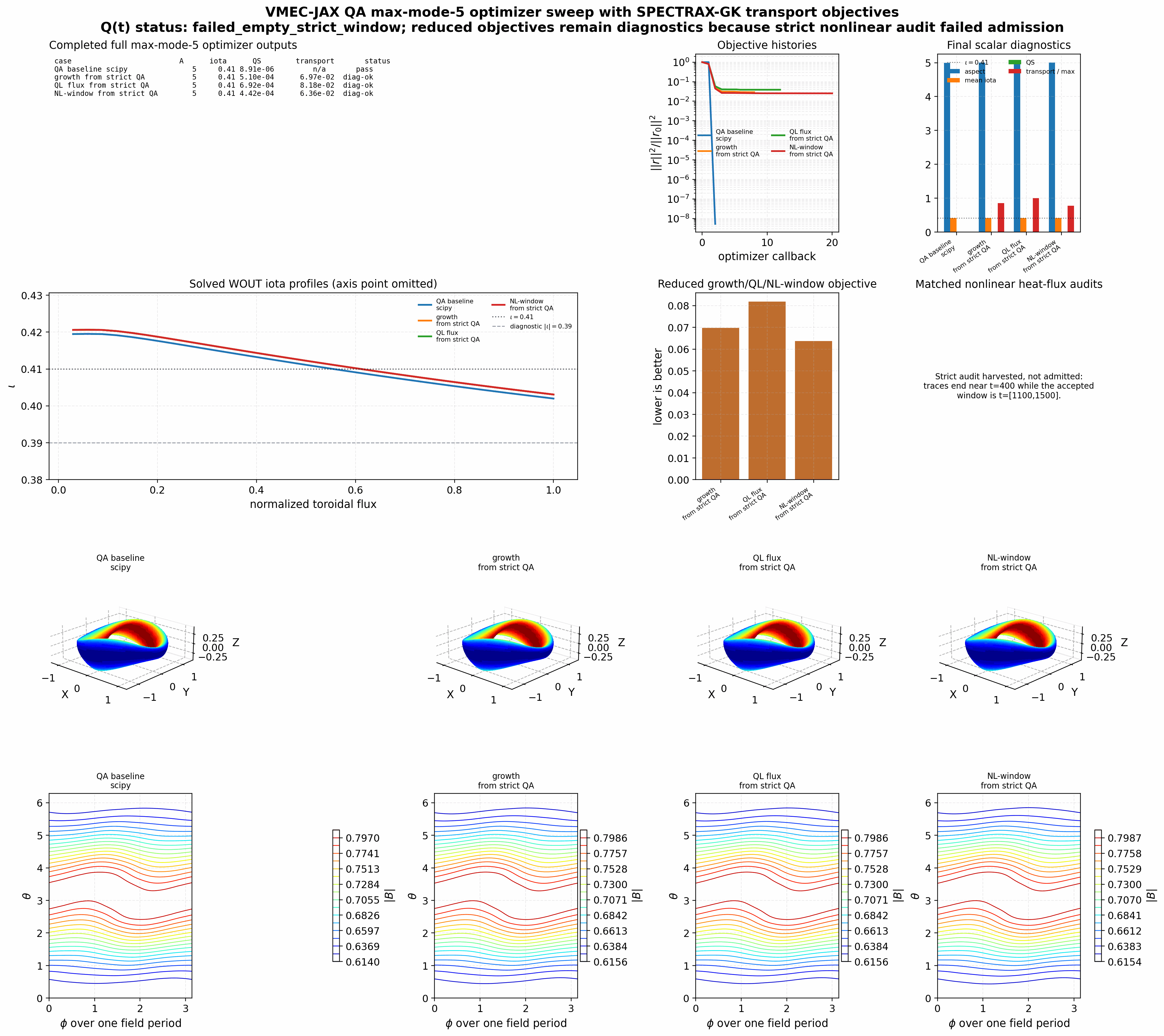
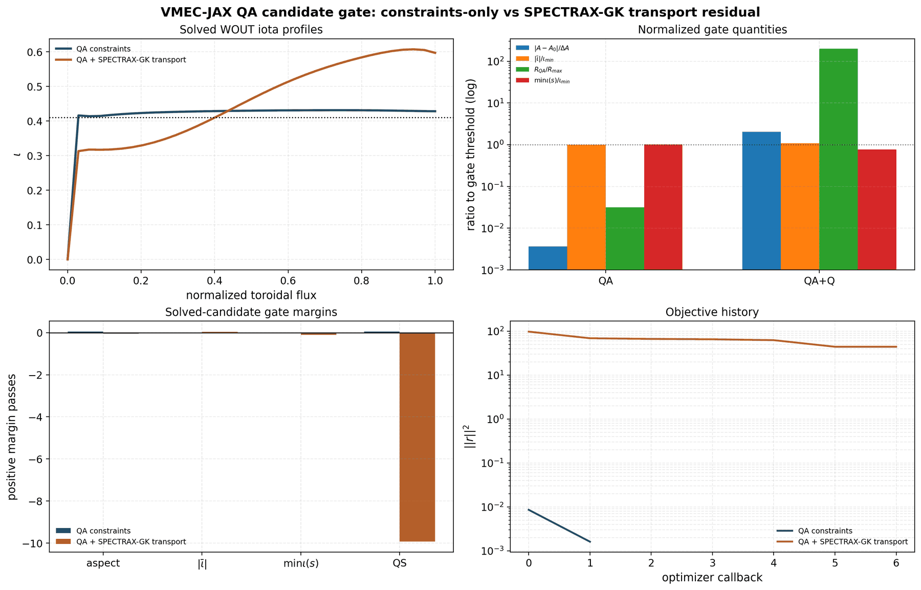
The panel builder compares the upstream-style QA baseline plus any completed growth-rate, quasilinear-flux, nonlinear-window, and projected/admission variants whose run directories are present. The current README-facing sweep uses the strict max-mode-5 QA baseline and three transport restarts from that baseline. It plots objective histories, solved-WOUT iota profiles, final aspect/iota/QS diagnostics, reduced transport metrics, 3-D LCFS surfaces colored by |B|, and LCFS |B| maps. It only plots nonlinear heat-flux traces when matched long-window GKX audit CSV files are present below the corresponding candidate directory.

This distinction is deliberate. The optimizer residual named nonlinear_window_heat_flux is a differentiable screening objective based on linear GKX rows and a smooth late-window envelope. It is useful for ranking candidate directions, but it is not a saturated turbulent heat-flux measurement. A candidate can be promoted to a nonlinear transport claim only after generating replicated post-transient GKX runs from its concrete wout_final.nc and demonstrating running-average convergence of Q(t). If a constraints-only QA baseline stops below the requested iota, increase the solve budget or use a small target buffer and rerun it. Do not promote it by relaxing the solved-WOUT gate; that would make later transport reductions depend on an inconsistent baseline. The configurable driver writes setup, history, input, and WOUT files. Physical admission remains a separate validation step because optimizer convergence is not a transport-convergence result. The tracked exact SciPy/ESS strict-baseline evidence is stored in docs/_static/vmex_qa_strict_baseline/summary.json. It terminates at nfev = 39 with aspect 5.000154, mean iota 0.4101997, QS residual 2.60e-4, and a passed solved-WOUT gate. The iota-profile floor is disabled for this baseline because the upstream QA_optimization.py objective uses a high-weight mean-iota target, not a profile-floor constraint. The older tracked strict-baseline artifact predates the current VMEC-JAX API and exposed an input/WOUT replay discrepancy. It remains useful negative evidence, but its removed command-line switches are not emulated. New campaigns must independently solve input.final, compare the replayed WOUT with the optimizer WOUT, and use only the authoritative replay for downstream transport audits.

Full max_mode=5 optimizer-output sweep from the office GPU node. The admitted constraints-only row follows the upstream VMEC-JAX QA simple-seed setup and passes the strict aspect/iota/QS gate. The growth, quasilinear, and nonlinear-window transport rows restart from that solved QA input. Their strict solved-WOUT gate is tripped by a small mean-iota shortfall, so the figure treats them as diagnostic-only non-admitted candidates rather than promoted optimized stellarators. The subsequent matched office audit is now harvested but still not admitted: its traces stop near t=400, outside the strict t=[1100,1500] acceptance window. The Boozer-LCFS |B| panels use unfilled contours so departures from quasisymmetry remain visible without a filled density map.

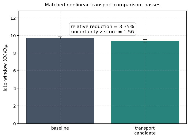
Matched single-point nonlinear transport audit for the full max-mode-5 projected weight 1e-3 candidate. Both baseline and candidate seed/timestep ensembles pass their individual long-window gates. The candidate lowers the late-window mean ion heat flux from 9.695 to 9.370: a 3.35% reduction with uncertainty separation z=1.56. The projected weight 5e-4 candidate also passes with 2.68% reduction. These are scoped single-surface, single-field-line, single-k_y positive audits, not broad stellarator-optimization claims. These matched nonlinear traces are tied to the earlier sweep baseline. The later 18-point matrix campaign against the strict max-mode-5 baseline failed for both projected-weight families, so the single-point positives remain candidate-screening evidence only.

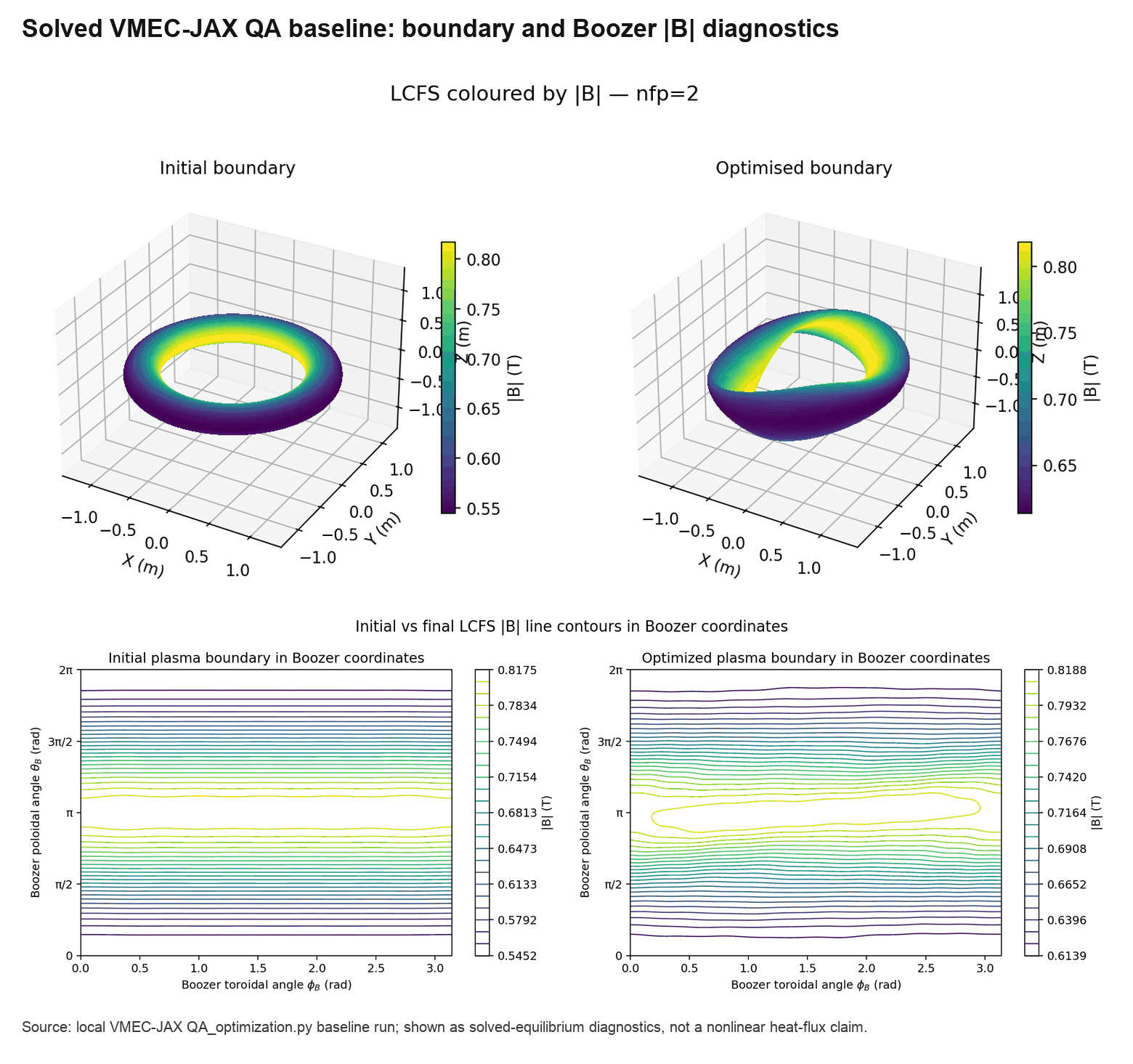
Solved VMEC-JAX QA baseline diagnostic generated from the local QA_optimization.py workflow. The top row compares initial and optimized LCFS surfaces colored by |B|; the bottom row shows the corresponding Boozer-LCFS |B| contours. This is the figure to use when discussing the solved QA baseline geometry. It is not a nonlinear heat-flux optimization claim.

Development-Only Reduced Diagnostics

The reduced max-mode-1 scripts are development diagnostics for AD/finite- difference checks, UQ plumbing, figure rendering, and sample-set reducers. They are intentionally outside examples/optimization and should not be used as solved QA stellarator optimization evidence.

python examples/theory_and_demos/reduced_stellarator_itg/stellarator_itg_growth_optimization.py
python examples/theory_and_demos/reduced_stellarator_itg/stellarator_itg_quasilinear_flux_optimization.py
python examples/theory_and_demos/reduced_stellarator_itg/stellarator_itg_nonlinear_heat_flux_optimization.py
python examples/theory_and_demos/reduced_stellarator_itg/compare_stellarator_itg_optimizations.py

They run a reduced max-mode-1 QA control model and are deliberately fast enough for local tests and figure regeneration. They do not generate the upstream VMEC-JAX QA_optimization.py final WOUT, and their synthetic LCFS views must not be used as README or manuscript evidence for solved QA geometry.

The shared constrained residual is

\[||r(x)||^2 = w_A \left({A(x)-A_0 \over A_0}\right)^2 + w_\iota \left(\iota(x)-\iota_0\right)^2 + w_{QS} R_{QS}(x)^2 + w_R ||x||^2 + r_T(x)^2 ,\]

where x is the reduced max-mode-1 QA control vector. The transport residual r_T is one of:

• growth: the positive dominant ITG growth-rate observable gamma;

• quasilinear_flux: a mixing-length proxy proportional to gamma Q_i / <k_perp^2> with tracked saturation metadata;

• nonlinear_heat_flux: the late-window mean of the differentiable envelope

  \[{dE \over dt} = 2\gamma E - \alpha E^2,\qquad Q_{\rm env}(t) = W_i E(t).\]

The comparison artifact docs/_static/stellarator_itg_optimization_comparison.png shows objective histories, reduced nonlinear Q_{\rm env} scans, fixed-gradient traces, reduced LCFS |B| surfaces, and reduced Boozer-coordinate LCFS |B| maps. These are reduced visualization diagnostics, not solved VMEC WOUT surfaces; in particular, the synthetic surface can look nearly axisymmetric when the reduced helical-control amplitude is small.

Solved QA Transport Optimization

The production workflow starts from the current VMEC-JAX precise-QA seed and adds one validated GKX transport objective while retaining the aspect, iota, and quasisymmetry residuals. Candidate equilibria remain unpromoted until solved-WOUT geometry gates and matched long-window nonlinear audits pass. This preserves the fixed-boundary equilibrium and precise-QA conventions of [HirshmanWhitson83] and [LandremanPaul22].

The solved-boundary VMEC-JAX path assembles the objective from in-memory VMEC states and requires the optional vmex and booz_xform_jax packages. It first solves a constraints-only QA baseline and then restarts a transport-weighted branch from that solved input. The current VMEC-JAX least-squares implementation owns the optimizer. GKX selects only the derivative policy appropriate to the observable; it no longer maintains a parallel optimizer-method abstraction.

The two branches use the upstream simple-seed perturbation and explicit mode continuation. The GKX study targets A=6 and mean iota=0.42; a passed optimizer run is still only a candidate. The required next audit is an independent WOUT profile/replay check followed by matched, replicated, long-window nonlinear heat-flux comparisons of baseline and candidate equilibria.

The A=6 admission artifact records mean_iota_lower_bound and iota_profile_floor fields. Legacy target_* iota fields remain in the JSON only as compatibility aliases and should be interpreted as lower-bound admission gates, not as the upstream QA script’s exact mean-iota objective.

Bounded VMEC-JAX solved-boundary plumbing audit. Admission is fail-closed: only a final authoritative solved_wout_gate.json can place a candidate in the expensive long-window nonlinear audit queue. Gates reconstructed from history.json plus wout_final.nc are recorded as advisory diagnostics only, because scalar histories can mix optimizer-residual and VMEC-state conventions. The current refreshed campaign admits the QA-only branch and blocks the scalar transport-weight refinement until a constraint-preserving/projection admission method produces a solved WOUT that keeps the aspect, profile-iota, and quasisymmetry margins.

The compact release contract at benchmarks/references/gkx_1_7_release_contract.json records the exact claim boundary and normalized prelaunch rows without duplicating the scientific figures. It keeps the max-mode-5 QA baseline, matched replicated nonlinear audit, and negative weak-margin control distinct: a raw audit pass is accepted only at the expected claim level with finite comparison metrics. The direct scalar transport branch and universal absolute-flux model remain blocked. The refreshed strict-baseline RBC(1,1) landscape is documented separately below and needs matched nonlinear ensemble sidecars before entering this admission policy.

Historical Projected-Gradient Evidence

The projected-gradient, frozen-axis boundary-chain, and guarded-weight tools used for the following tracked artifacts targeted a VMEC-JAX optimizer API that has since been removed. They are no longer shipped as runnable campaign tools: emulating that object model would create a second equilibrium/optimizer stack and an ambiguous derivative convention. The JSON sidecars and figures remain as historical negative and conditioning evidence.

New campaigns use current VMEC-JAX opt.least_squares directly. Growth-rate optimization uses its implicit equilibrium Jacobian and must pass the local GKX eigenbranch/tangent gates; eigenvector-weighted QL and reduced nonlinear objectives use finite-difference outer Jacobians. Candidate boundaries are replayed independently and evaluated before any matched nonlinear audit. This current path replaces the former private fixed-boundary stage, manual frozen-axis tape access, and projected-input writer.

The historical multicomponent audit found internally consistent frozen-axis JVP/VJP contractions but branch-sensitive exact-solve differences for some coefficients. The accepted projected step reduced its reduced single-sample metric but did not reduce the matched long-window nonlinear flux. Those results remain important guardrails: internal transpose consistency is insufficient, and reduced local objective descent is not a turbulent-transport claim.

VMEC-JAX/GKX transport-gradient line-search audit. Green points pass the solved-equilibrium aspect, iota, and QS gates; the red point is rejected by the QS gate. The best accepted projected step reduces the reduced transport metric by 3.55% and defines the candidate for the next matched long-window nonlinear audit.

The matched long-window nonlinear audit for that earlier aspect-6 admitted projected candidate has now been run at the production n64 grid with two seed replicates and one timestep replicate over t=[350,700]. Both the baseline and projected candidate ensembles pass their individual stationarity/replicate gates, but the matched comparison does not promote the projected step: the baseline late-window mean ion heat flux is 9.833 while the projected candidate is 9.891. The relative reduction is therefore -0.00585 with a combined uncertainty of 0.293 and uncertainty z-score -0.20. This closes the first projected-candidate audit as a negative transfer result: the reduced single-sample transport metric is locally differentiable and useful for admission, but it did not predict a statistically resolved lower long-window nonlinear flux for this boundary step.

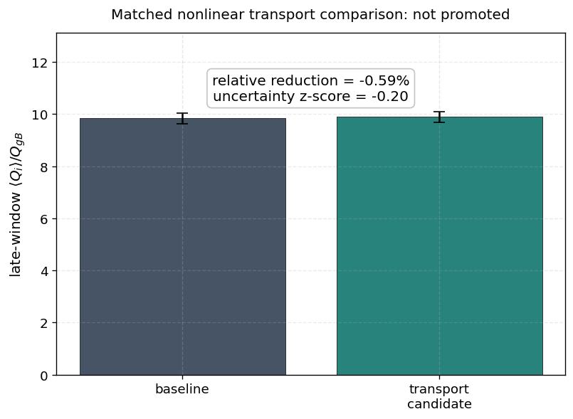
Matched replicated nonlinear transport comparison for the accepted projected QA boundary step. Each bar is a passed t=[350,700] seed/timestep ensemble. The projected candidate is not promoted because its ensemble mean is slightly higher than the baseline within uncertainty.

The redesign gate in docs/_static/qa_projected_transport_step1e3_redesign_report.json converts this negative audit into the next objective contract. It blocks promotion on insufficient_matched_reduction, insufficient_uncertainty_separation, and under-resolved single-point objective coverage. The recommended next reduced objective evaluates 3 x 2 x 3 = 18 points: surfaces s = (0.45, 0.64, 0.78), field-line labels alpha = (0, pi/4), and grid-compatible k_y rho_i = (0.10, 0.30, 0.50). Future projected candidates must pass that multi-sample reduced admission before another expensive matched nonlinear audit is scientifically justified. The later strict top-12 QA edge candidate does pass this 18-point reduced coverage and lowers the reduced metric by 2.29%, but its matched t=[350,700] nonlinear audit still fails promotion: the relative reduction is only 0.58% with uncertainty z-score 0.20. Its docs/_static/strict_qa_top12_edge_redesign_report.json artifact therefore keeps the nonlinear turbulent-flux optimization claim blocked until the reduced objective has stronger predictive margin and uncertainty-aware admission. The companion strict_qa_top12_edge_prelaunch_gate.json records the same lesson as a prelaunch rule: the 2.2876% reduced margin is below the 4% calibrated threshold, so a future candidate at this margin would be blocked before launching a new expensive nonlinear campaign.

The broad nonlinear turbulent-flux optimization gate is a full production campaign over s=(0.45,0.64,0.78), alpha=(0,pi/4), and k_y rho_i=(0.10,0.30,0.50) with seed/timestep replicated t=[1100,1500] nonlinear windows. Its postprocess rebuilds every output gate, ensemble gate, matched comparison, and the aggregate matrix report. A broad optimization claim is allowed only when that aggregate report passes; otherwise the candidate remains single-point or diagnostic evidence. If several candidate families are available, the final release decision is made by tools/release/check_nonlinear_transport_gates.py matrix-portfolio. It consumes one or more aggregate matrix reports, selects the passing family with the largest mean heat-flux reduction, and records strict t=1500 growth/QL/nonlinear-window matched comparisons only as excluded negative-transfer evidence. Only a passing portfolio is eligible for the publication figure command. The portfolio JSON and selected matrix report remain the authoritative evidence; blocked portfolios are never copied into the release figure index.

Boundary-Coefficient Objective Landscapes

Before launching another optimizer, GKX now includes a boundary-coefficient landscape diagnostic. It perturbs one VMEC input coefficient, writes the corresponding input.* decks, evaluates deterministic reduced transport objectives, and optionally overlays true post-transient nonlinear heat-flux points with uncertainty bars. This mirrors the optimization lesson in [Kim24]: time-averaged nonlinear heat flux can be noisy enough that local deterministic descent may fail near a minimum, so the optimizer choice should be informed by a pre-optimizer landscape scan.

The current RBC(1,1) diagnostic starts from the strict max-mode-5 QA baseline used in the optimizer sweep and scans the coefficient over [-75%, +75%] with 31 points. The top panel evaluates the linear growth rate and every explicit electrostatic quasilinear heat-flux rule on the same multi-point optimizer sample set: s = (0.45, 0.64, 0.78), alpha = (0, pi/4), and k_y rho_i = (0.10, 0.30, 0.50). The lower panel is deliberately not a reduced nonlinear-window objective. It accepts only long-window post-transient nonlinear heat-flux ensemble sidecars produced from concrete GKX nonlinear outputs. This separation is part of the claim boundary: reduced/startup nonlinear-window diagnostics can guide launch choices, but they cannot be plotted or cited as turbulent heat-flux landscapes.

The reduced scan is intentionally reusable. The batched evaluator computes growth and all explicit quasilinear metrics in one VMEC/JAX solve per coefficient; reduced/startup nonlinear-window metrics are excluded from this landscape.

When selected landscape points are promoted to expensive turbulence evidence, run replicated post-transient nonlinear ensembles and rerun the plot with --nonlinear-ensemble coefficient_value:path/to/ensemble.json. Only those ensemble sidecars should feed uncertainty-aware nonlinear admission reports. For the current strict-baseline RBC(1,1) scan, the paper-facing nonlinear protocol is t_max = 1500 with the accepted transport window t = [1100, 1500] on the n64:64:64:40:40 grid. The earlier t = [350, 700] pilot for the -75% point remained visibly transient and failed running-mean convergence. A neighboring -70% point passed readiness but failed timestep-spread robustness over t = [700, 1100] and then passed over t = [1100, 1500]. The tracked public overlay currently includes 24 coefficients that have passed the accepted diagnostic t = [1100, 1500] seed/timestep ensemble gate: the negative side, the zero-offset baseline, and eight positive coefficients, +5%, +10%, +15%, +20%, +25%, +30%, +35%, and +40%. The +20% coefficient is a scoped relaxed diagnostic admission: its mean-relative seed/timestep spread is 15.48%, so it passes the explicitly selected 20% landscape gate but not the stricter 15% production-style gate. The remaining higher positive coefficients are stability-boundary/open long-window points and should not be inferred from reduced metrics. The shorter windows are retained only as negative convergence diagnostics for this landscape protocol.

Earlier +3% RBC(0,1) and sparse RBC(1,1) sidecars are retained as historical development artifacts only. They were generated from older narrow or reduced screening scans and should not be interpreted as admission reports for the current strict-baseline [-75%, +75%] figure.

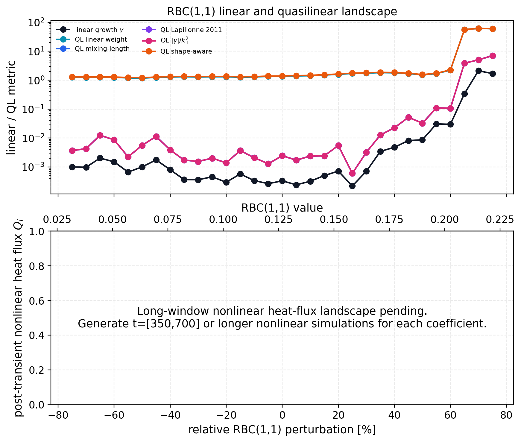
RBC(1,1) transport-objective landscape from the strict max-mode-5 QA baseline. The top panel shows linear growth and the shipped quasilinear rules. The bottom panel is true nonlinear heat flux only when populated by long post-transient ensemble sidecars; reduced nonlinear-window diagnostics are excluded from this figure.

Current VMEC-JAX WOUT files provide Aminor_p, Rmajor_p, aspect, and volume_p from the solved equilibrium. GKX consumes those values directly; the runtime EIK path rejects an invalid Aminor_p. In-memory bridge workflows may instead pass an explicit reference length for normalization. GKX does not estimate or rewrite equilibrium scalars from the LCFS boundary.

Implementation Map

• Legacy nonlinear landscape admission report from the earlier narrow scan: vmec_boundary_transport_landscape_admission.json

• Legacy reduced nonlinear-audit prelaunch gate from the earlier narrow scan: vmec_boundary_transport_prelaunch_gate.json

• Legacy nonlinear optimizer campaign-admission gate from the earlier narrow scan: nonlinear_campaign_admission_report.json

VMEC-JAX Geometry Examples

The user-facing VMEC geometry examples are WOUT-backed runtime workflows. They use small vmex input decks shipped under examples/vmec and avoid separate EIK generation for the common demo path:

pip install vmec-jax
cd examples/vmec
./generate_wouts.sh
cd ../..

gkx run --config examples/linear/axisymmetric/runtime_circular_vmec_linear.toml
gkx run --config examples/linear/non-axisymmetric/runtime_hsx_linear_quasilinear.toml
gkx run --config examples/linear/non-axisymmetric/runtime_w7x_linear_quasilinear_vmec.toml

Run vmex input.NAME inside examples/vmec when only one WOUT is needed. These bundled QHS/QI/QA decks are self-contained demonstration equilibria. Machine-specific HSX or W7-X validation should use the same TOMLs with --vmec-file pointing to the benchmark WOUT.

This disk-WOUT path is the runtime example path, not the production optimizer gradient contract. The production optimizer starts from an in-memory solved vmex state, transforms through booz_xform_jax, and then builds the GKX flux tube without relying on intermediate NetCDF files.

Production VMEC-JAX Optimization Plan

The production lane starts from the vmex fixed-boundary QA optimizer: aspect ratio is constrained, the mean rotational transform uses the original VMEC-JAX high-weight MeanIota target by default, the quasisymmetry residual is penalized, and a GKX transport objective is added as another residual block. The default paper-facing seed now targets A = 6 and iota = 0.41 at a fixed ITG flux tube, initially torflux = 0.64 and alpha = 0.0. A one-sided floor mode remains available for experiments, but the target mode is the default because it prevents the low-signed-mean-iota failure observed with the absolute-floor smoke. The optimized result must also pass held-out field-line and surface gates before any stellarator-wide claim.

A bounded VMEC-JAX smoke run has been checked with max_mode=1, mboz=nboz=21, a GKX growth residual, and a single scalar-trust evaluation. It assembled the four residual blocks (aspect, absolute-iota floor, quasisymmetry, GKX transport) and retained the iota floor with min |iota| = 0.410000 and mean iota 0.481850. This validates the in-memory optimizer hook and iota-floor convention; it is not yet the final transport-aware optimized equilibrium used for a turbulence claim.

The public VMEC-JAX QA transport scripts are:

• QA_optimization_linear_ITG.py: append a GKX ITG growth-rate objective to the upstream QA/aspect/iota tuple list.

• QA_optimization_quasilinear_ITG.py: append a quasilinear transport diagnostic objective to the same solved-equilibrium optimization.

• QA_optimization_nonlinear_ITG.py: append a nonlinear-window heat-flux screening objective, then promote only if matched baseline and optimized equilibria pass replicated long-window post-transient heat-flux audits.

Development-only reduced diagnostics remain under examples/theory_and_demos/reduced_stellarator_itg for AD/FD and plotting tests; they are not production QA optimization examples.

For the geometry layer, the user-facing runtime examples use WOUT files generated from the small examples/vmec/input.* decks with vmex. The optimizer path should avoid disk I/O: it should pass a solved vmex state through booz_xform_jax with mboz >= 21 and nboz >= 21, then into the GKX flux-tube contract. Disk WOUTs remain useful for reproducibility, release artifacts, and external benchmark comparison.

Every promoted optimization figure needs a sidecar JSON/CSV artifact and a gate:

• objective history and coefficient trajectory;

• before/after Boozer |B| contours and quasisymmetry residuals;

• before/after growth-rate spectra;

• before/after quasilinear spectra with uncertainty intervals;

• nonlinear heat-flux time traces with transient cut, running mean, block/SEM uncertainty, and replicate spread;

• AD-vs-finite-difference gradient parity and sensitivity/covariance maps;

• Pareto plot of quasisymmetry residual, aspect/iota constraint error, and transport reduction.

The nonlinear heat-flux optimizer must not use startup or reduced-window values as final evidence. Production evidence requires long post-transient averages whose running means are converged and whose seed/timestep/grid replicates agree within the documented gate.

The broad matched baseline/candidate matrix over three surfaces, two field lines, and three k_y values is the multi-surface promotion artifact: all baseline/candidate ensembles must pass their long post-transient window gates, and the matched comparison matrix must satisfy the configured pass-fraction and mean-reduction policy. After postprocessing candidate families, use the portfolio gate to pick the promoted family and to keep strict negative-transfer rows out of the promotion count:

python tools/release/check_nonlinear_transport_gates.py matrix-portfolio \
  --matrix-report accepted_qa_ess=tools_out/qa_ess_matrix/artifacts/qa_ess_matrix_report.json \
  --matrix-report projected_0p001=tools_out/projected_0p001_matrix/artifacts/projected_0p001_matrix_report.json \
  --excluded-comparison strict_growth=docs/_static/vmec_qa_t1500_baseline_to_growth_comparison.json \
  --excluded-comparison strict_quasilinear=docs/_static/vmec_qa_t1500_baseline_to_quasilinear_comparison.json \
  --excluded-comparison strict_nonlinear_window=docs/_static/vmec_qa_t1500_baseline_to_nonlinear_window_comparison.json \
  --out-json tools_out/nonlinear_transport_matrix_portfolio.json \
  --out-figure tools_out/nonlinear_transport_matrix_portfolio.png

Development Portfolio Gate

Before the VMEC/Boozer optimizer is promoted, the same reducer used by the future production objective is exercised on a cheap differentiable sample table. The table is rectangular in normalized toroidal flux, field-line alpha, and k_y rho_i. The default gate covers three surfaces, two field-line alpha values, and three k_y values with growth-rate and quasilinear-flux columns. It checks both the scalar reduced objective and every unreduced row against central finite differences.

python examples/theory_and_demos/reduced_stellarator_itg/stellarator_itg_portfolio_gate.py \
  --finite-difference-workers 2

By default this writes docs/_static/stellarator_itg_portfolio_gate.{json,png,pdf}. Use --surfaces, --alphas, --ky-values, and --objectives only when the changed sample set is also recorded in the artifact sidecar. The JSON sidecar is the audit source: it records claim_level, sample_set, backend_boundary, scalar/row-wise pass status, and the reduced objective table. The PNG/PDF are human-readable renderings of that sidecar, not separate validation evidence.

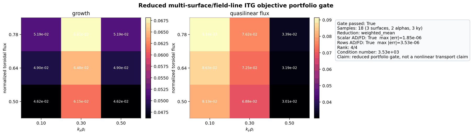
Reduced multi-surface/field-line ITG objective portfolio gate. The heatmaps show the alpha-averaged growth and quasilinear-flux objective rows across three surfaces and three k_y values. The side panel records scalar and row-wise AD/finite-difference agreement, full-rank sensitivity, and the explicit claim boundary: this is a reduced portfolio gate, not a nonlinear turbulent-transport optimization claim.

The production bridge now uses the same portfolio layout for real vmex -> booz_xform_jax -> GKX row production: stellarator_itg_vmec_boozer_sample_objective_table_from_state evaluates physical toroidal-flux, field-line alpha, and k_y rho_i samples, while stellarator_itg_vmec_boozer_portfolio_objective_from_state applies the same weighted reducer. The aggregate VMEC/Boozer artifact tool accepts physical --ky-values and records the resolved solver indices, Ly, Ny, and per-sample ky_abs_error in the sidecar. The remaining promotion step is scientific, not plumbing: rerun held-out surface/field-line gates and promote nonlinear candidates only after long post-transient replicated windows pass for matched baseline and optimized equilibria.

For CI-scale development, solver_objective_branch_gradient_report applies the same branch-continuity and implicit AD/finite-difference logic to the solver-ready differentiable geometry contract. It verifies that the selected max-growth eigenbranch stays dominant under central perturbations and that the objective-vector sensitivities pass the implicit left/right eigenpair gate. The VMEC/Boozer offline gates remain the authority for production stellarator optimization claims.

Optimizer drivers should use vmec_boozer_scalar_objective_from_state once they have a solved vmex state. The supported aliases are growth/gamma, frequency/omega, and quasilinear_flux/mixing_length_heat_flux_proxy. This selector prevents each optimization example from silently using a different objective index.

The production-facing geometry objective should not stay tied to one field line or one k_y point. vmec_boozer_solver_objective_table_from_state evaluates the same solver-objective vector over explicit surface_indices, field-line alphas, and selected_ky_indices and returns the full table before any reduction. vmec_boozer_aggregate_scalar_objective_from_state then reduces that table with a mean, weighted mean, or worst-case max. Mean and weighted mean are the preferred gradient-development targets because the sample set is fixed. A max reduction is useful as a conservative diagnostic, but it must not be treated as a smooth optimizer objective unless active-set and branch-continuity diagnostics are also passed.

Before any optimizer loop is promoted, run vmec_boozer_scalar_objective_finite_difference_report on the selected VMEC coefficient, field line, and objective. It evaluates the scalar objective at x-h, x, and x+h through the same in-memory VMEC/Boozer path and records the central finite-difference sensitivity. The report also checks a curvature/branch-switch indicator so a non-smooth max-growth branch is not mistaken for a usable optimization gradient. This is intentionally a finite-difference/SPSA-compatible audit, not an automatic-differentiation claim for eigenvector-dependent quasilinear observables.

For multi-surface or multi-k_y objectives, run vmec_boozer_aggregate_scalar_objective_finite_difference_report with the same sample set and weights used by the optimizer. The report records the sample metadata, scalar values, objective tables, and the same curvature/branch-switch indicator. This is the minimum gate before a stellarator optimization study can claim that a reduced growth-rate or quasilinear objective decreased across more than one field line, surface, or k_y point.

The first optimizer scaffold is vmec_boozer_scalar_objective_line_search_report. It repeatedly applies the finite-difference audit at the current VMEC coefficient offset and accepts only candidate updates that both pass the same curvature gate and reduce the scalar objective. This is useful for growth-rate and quasilinear-flux optimizer plumbing, but it remains a one-parameter audit rather than a multi-parameter stellarator optimization claim.

For multi-point reduced objectives, use vmec_boozer_aggregate_scalar_objective_line_search_report instead. It applies the aggregate finite-difference gate at every attempted VMEC coefficient update and records the same sample metadata as the aggregate gate. This is now the preferred scaffold for growth-rate and quasilinear-flux optimization studies that need more than one field line, surface, or k_y point before entering a full optimizer loop.

Training improvement is not enough for a geometry-wide claim. vmec_boozer_aggregate_line_search_holdout_report runs the same aggregate line-search on a training sample set, then evaluates the final coefficient offset on a disjoint held-out sample set. The split gate passes only if both the training line-search gate and held-out aggregate reduction pass. This is the minimum reduced-objective validation step before using an optimized VMEC coefficient in manuscript figures.

Production promotion adds a stricter surface/field-line rule. The aggregate finite-difference, line-search, and reduced holdout reports must be paired with at least one separate passed validation artifact whose sample metadata covers a held-out surface_index or field-line alpha. A held-out k_y point alone is useful spectrum coverage, but it is not sufficient for the surface/field-line generalization gate. The repository-level check tools/release/check_vmec_boozer_gates.py aggregate-holdout encodes that boundary for frozen artifacts: it accepts the aggregate FD and line-search artifacts as necessary optimizer-plumbing evidence, then blocks promotion until independent surface/field-line holdout evidence is supplied. It also requires a passed replicated nonlinear-window ensemble artifact from tools/release/check_nonlinear_transport_gates.py ensemble before any optimized-equilibrium production nonlinear heat-flux claim can be made. The ensemble requirement is deliberately separate from the single-window convergence rule: a single post-transient mean can establish a candidate window, but seed/timestep/restart replicates are needed before that mean becomes a robust optimization target.

Objective

Let

\[p = \left[ \Delta \log a,\ \Delta \kappa,\ \epsilon_h,\ \Delta \hat{s} \right]\]

denote the four active max-mode-1 controls used by the examples: a minor-radius shift, vertical-elongation shift, helical-ripple amplitude, and magnetic-shear shift. The constrained objective is

\[J_k(p) = w_A \left(\frac{A(p) - A_*}{A_*}\right)^2 + w_\iota \left(\iota(p) - \iota_*\right)^2 + w_{QS} R_{QS}(p)^2 + w_r \|p\|_2^2 + w_T T_k(p),\]

with A_* = 7 and iota_* = 0.41. The turbulence term T_k selects one of three differentiable objectives.

Growth-rate objective:

\[T_\gamma(p) = \gamma(p).\]

Quasilinear heat-flux objective:

\[T_{QL}(p) = C_{sat}\, \frac{\gamma_+(p)\, W_i(p)} {k_{\perp,\mathrm{eff}}^2(p) + \epsilon},\]

where W_i is the linear heat-flux weight and gamma_+ is a smooth positive growth-rate part. This mirrors the mixing-length-style objective used in the quasilinear module and is a differentiable optimization proxy, not a promoted absolute-flux predictor. The current train/holdout quasilinear calibration pages show why absolute saturated-flux claims remain gated.

Nonlinear-window objective:

\[\frac{dE}{dt} = 2\gamma(p) E - \alpha(p) E^2, \qquad Q_i(t; p) = W_i(p) E(t; p),\]

integrated with a fixed-step RK2 update. The objective is the late-window average

\[T_{NL}(p) = \frac{1}{t_2 - t_1} \int_{t_1}^{t_2} Q_i(t; p)\,dt,\]

with companion quality metrics

\[C_V = \frac{\mathrm{std}(Q_i)}{|\langle Q_i \rangle|}, \qquad \mathrm{trend} = \frac{|dQ_i/dt| (t_2-t_1)} {|\langle Q_i \rangle|}.\]

The nonlinear objective is intentionally an envelope gate. It is useful for testing differentiable late-window averaging and optimizer behavior before the full nonlinear GK RHS is promoted into an end-to-end differentiated objective.

Numerics and Differentiation

The optimizer uses JAX reverse-mode gradients through the scalar objective and a bounded Adam update with clipped controls. Every shipped artifact records:

• the full objective history;

• the parameter and observable histories;

• an autodiff-vs-central-finite-difference Jacobian report;

• a Gauss-Newton covariance diagnostic from the final weighted objective residual Jacobian;

• for the nonlinear-window objective, the initial and optimized heat-flux traces, averaging window, coefficient of variation, and trend.

The finite-difference gate is

\[\max_{ij} |J^{AD}_{ij} - J^{FD}_{ij}| < \epsilon_{abs} \quad\mathrm{or}\quad \frac{|J^{AD}_{ij} - J^{FD}_{ij}|}{|J^{FD}_{ij}| + \epsilon} < \epsilon_{rel},\]

with tighter tolerances when JAX x64 is enabled.

Small geometry and objective-observable checks should use the shared observable_gradient_validation_report helper. The helper reports finite flags, absolute and relative AD/finite-difference errors, tangent-direction agreement, rank, singular values, condition number, and a pass/fail gate in a strict JSON-compatible payload. The tiny solver-ready objective gate in The focused objective owners exposed through gkx exercise this path without running VMEC, Boozer, or a linear eigenproblem; it is a CI and documentation check for the reporting contract, not a transport-gradient claim.

For the VMEC/Boozer bridge reports, passing this AD/FD tolerance is necessary but not sufficient for optimization readiness. The geometry sensitivity reports also carry a conditioning block with singular values, numerical rank, condition number, AD row/column norms, per-parameter finite-difference step scaling, and the worst error location. This keeps three cases separate in the artifacts: a failed derivative implementation, a correct but ill-conditioned control direction, and a well-conditioned reduced optimization gate. The current full-chain vmex state-coefficient reports should therefore be read as reduced linear/quasilinear/nonlinear-window estimator differentiability evidence until converged nonlinear heat-flux gradients or optimized-equilibrium finite-difference audits also pass.

The UQ diagnostic uses the weighted residual vector whose squared norm is the reported objective:

\[r = \left[ \sqrt{w_A}\frac{A-A_*}{A_*},\ \sqrt{w_\iota}(\iota-\iota_*),\ \sqrt{w_{QS}}R_{QS},\ \sqrt{w_r}p,\ \sqrt{w_T T_k} \right].\]

The local covariance is then

\[C_p = \sigma^2 \left(J_r^T J_r + \lambda I\right)^{-1},\]

where J_r = dr/dp and sigma^2 is estimated from the final residual. This is intentionally tied to the optimization objective. It is not computed from the initial-to-final parameter displacement, which would measure optimizer travel rather than local uncertainty at the optimized point.

Objective-portfolio artifact guard

Multi-surface, multi-field-line, and multi-k_y stellarator studies should separate two contracts:

• row production, where VMEC/Boozer/GKX evaluates one objective vector per sample;

• row reduction, where those fixed samples are combined into one scalar for an optimizer or UQ ensemble.

The reducer in gkx.objectives.portfolio requires a real numeric (surface, alpha, ky, objective) table, finite non-negative normalized weights, and an explicit reduction policy. Its unit tests cover shape, weighting, JVP, reverse-mode, and finite-difference contracts. The research-facing evidence is the real-artifact guard tools/release/check_vmec_boozer_gates.py reduced-portfolio. It consumes the tracked multi-alpha VMEC/Boozer aggregate-objective JSON plus a VMEC/Boozer AD/FD gradient JSON, rebuilds a backend-free reducer table from the real rows, and fails closed unless the artifact has VMEC/Boozer provenance, at least two field-line alpha values, at least two k_y samples, finite FD and AD/FD diagnostics, growth and quasilinear objective columns, and an explicit non-production nonlinear claim boundary.

python tools/release/check_vmec_boozer_gates.py reduced-portfolio

The tracked guard lives at docs/_static/vmec_boozer_reduced_portfolio_guard.json and passes on the QH mode-21 multi-alpha/two-k_y artifact. It admits reduced growth/QL portfolio plumbing only; production nonlinear turbulent-transport optimization now additionally requires the separate optimized-equilibrium long-window transport audit tracked below. That audit is closed for the selected QA candidate, while nonlinear turbulence gradients and broad multi-surface optimization remain separate gates.

Development Diagnostic Results

Generate the three individual optimization panels with:

JAX_ENABLE_X64=1 python examples/theory_and_demos/reduced_stellarator_itg/stellarator_itg_growth_optimization.py --finite-difference-workers 2
JAX_ENABLE_X64=1 python examples/theory_and_demos/reduced_stellarator_itg/stellarator_itg_quasilinear_flux_optimization.py --finite-difference-workers 2
JAX_ENABLE_X64=1 python examples/theory_and_demos/reduced_stellarator_itg/stellarator_itg_nonlinear_heat_flux_optimization.py --finite-difference-workers 2

Generate the comparison panel with:

JAX_ENABLE_X64=1 python examples/theory_and_demos/reduced_stellarator_itg/compare_stellarator_itg_optimizations.py --workers 3 --finite-difference-workers 2
JAX_ENABLE_X64=1 python tools/artifacts/plot_stellarator_optimization_uq.py

The --workers option parallelizes the independent growth-rate, quasilinear-flux, and nonlinear-window objective reports while preserving the serial ordering of the JSON payload. The --finite-difference-workers option parallelizes central finite-difference columns inside each AD/FD gate using threads, which avoids pickling JAX objective closures. Both paths record their worker metadata and identity contract in the JSON artifacts.

The development-only reduced comparison sidecar docs/_static/stellarator_itg_optimization_comparison.json records three differentiable QA-control ITG residuals from the same initial control vector. All three keep the reduced objective near A = 7 and iota = 0.41 while reducing the tracked transport observables. In the current artifact, the optimized growth rate is about 57% of the initial value and both quasilinear and nonlinear-window heat-flux observables are about 41% of their initial values. This is retained as model-development and AD/FD plumbing evidence only. Its companion rendered PNG is a synthetic max-mode-1 surface diagnostic that can look nearly axisymmetric when the reduced helical amplitude collapses; it is therefore not a paper-facing solved-geometry optimization figure. Use the solved VMEC-JAX QA boundary/Boozer panel above for baseline geometry visualization.

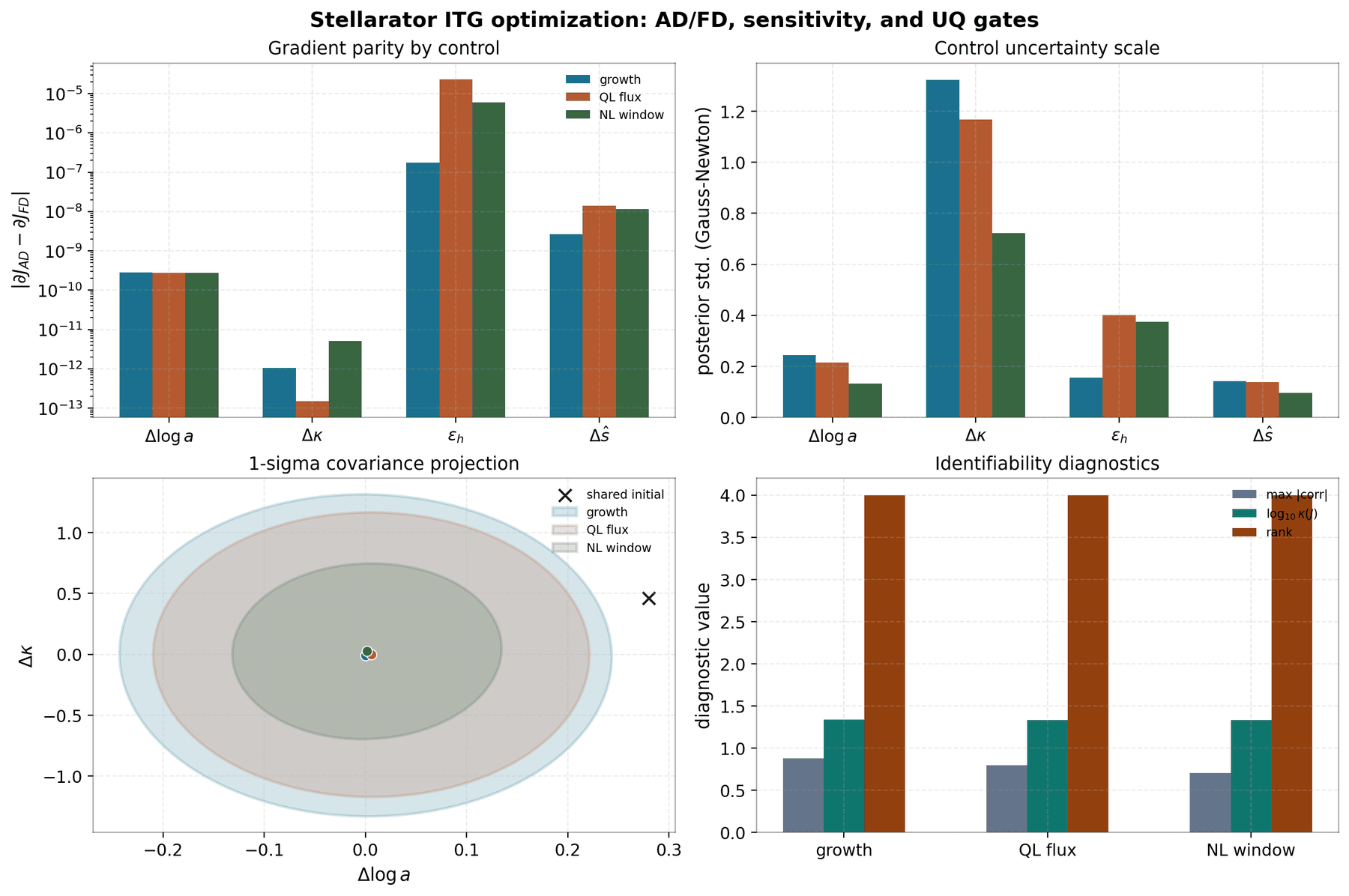
UQ and sensitivity diagnostics for the same three reduced objectives. The first panel verifies AD/FD derivative parity for every active control. The covariance panels use the weighted objective residual map above, so the reported uncertainty is a local identifiability diagnostic at the optimized point. All three reduced objectives remain full-rank and finite-difference checked in this artifact; the claim is still limited to optimization plumbing, not full VMEC/Boozer/GK nonlinear optimization.

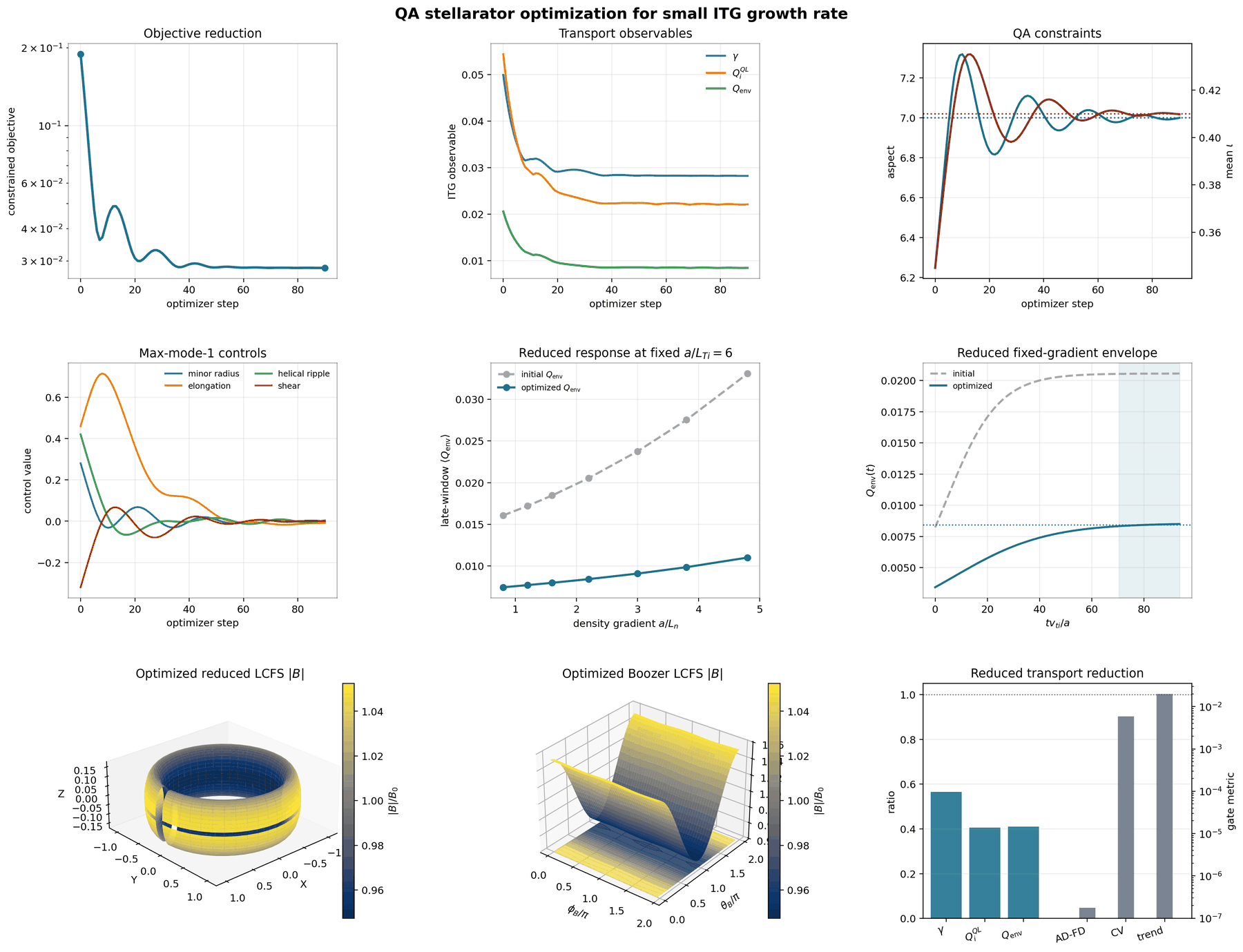
Growth-rate objective history, coupled transport observables, reduced a/L_n response, fixed-gradient Q_env trace, optimized reduced LCFS |B| surface, and reduced Boozer-LCFS |B| map. These geometry panels are reduced max-mode-1 diagnostics, not solved VMEC WOUT plots.

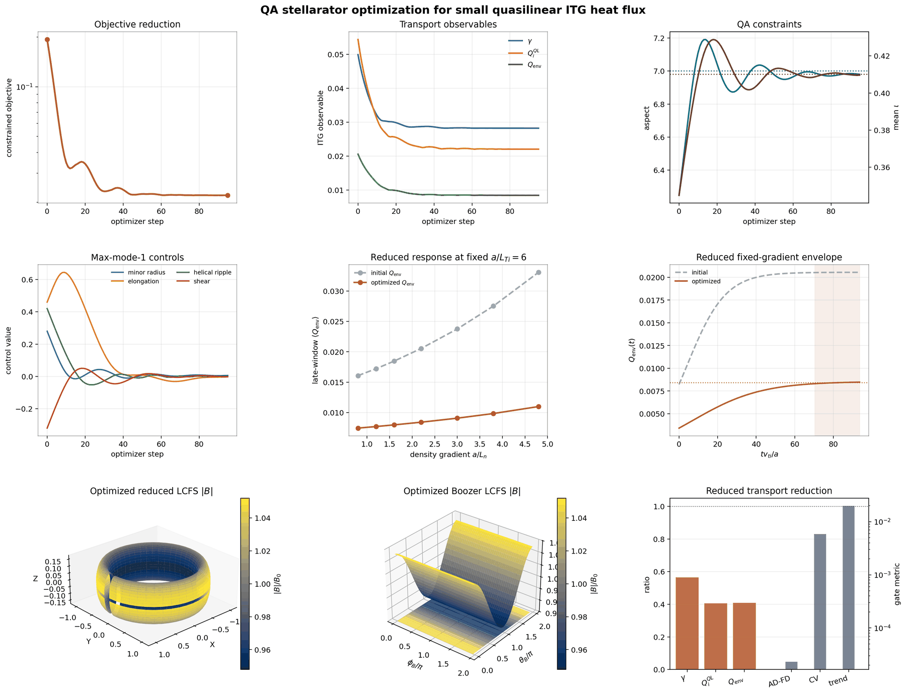
Quasilinear heat-flux objective history and the same reduced scan, trace, LCFS |B|, and Boozer-LCFS |B| diagnostics. The quasilinear objective uses the differentiable mixing-length feature map tested in Quasilinear Transport; it is still a reduced diagnostic, not a promoted absolute-flux predictor.

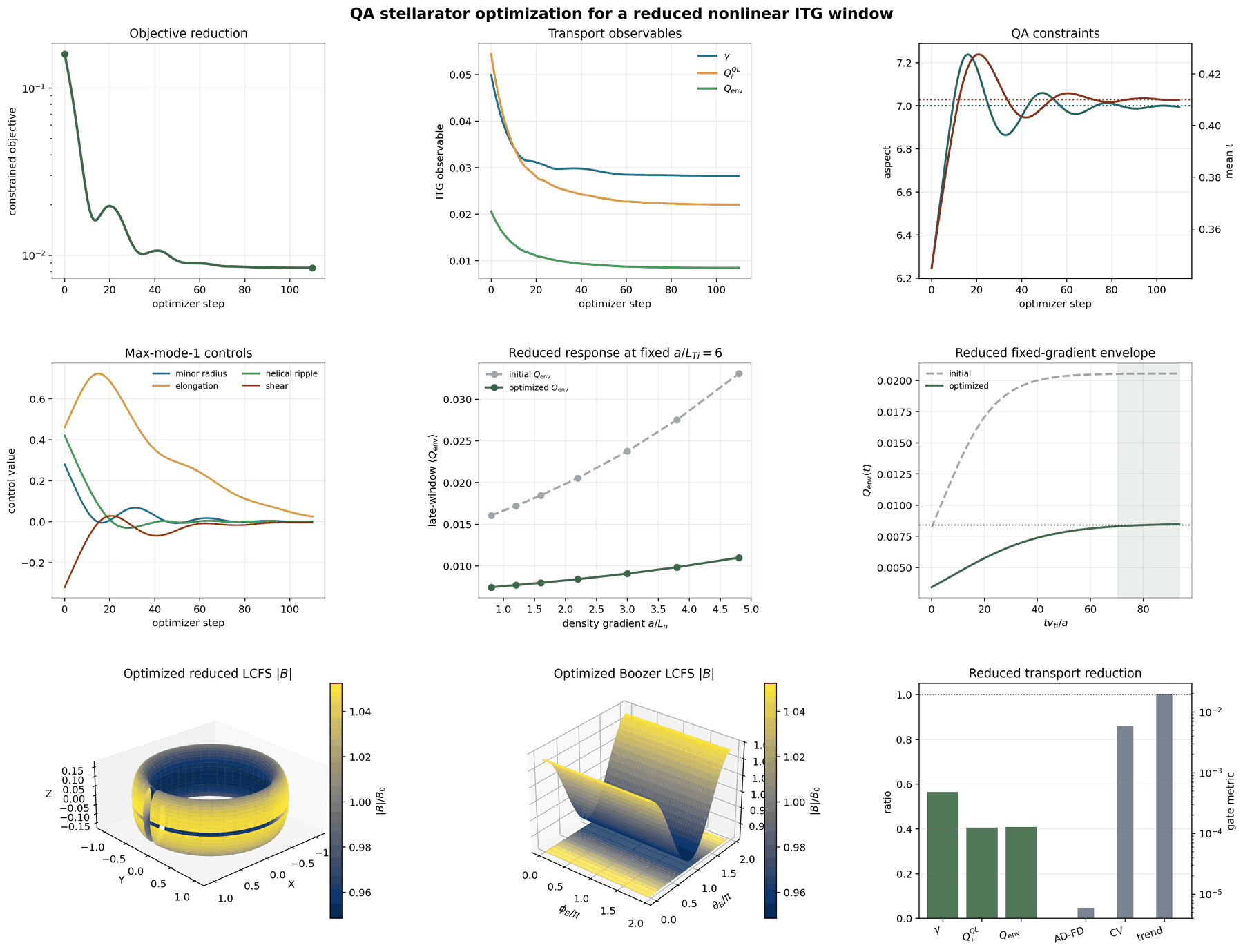
Reduced nonlinear-window objective history, fixed-gradient heat-flux envelope, reduced density-gradient response, and reduced LCFS/Boozer |B| diagnostics. The shaded region is the averaging window used in the objective. The shipped artifact records a low coefficient of variation and trend for the optimized late-time window, so the plotted average is meaningful for this reduced model; production turbulent-flux optimization still requires solved-WOUT nonlinear transport audits.

Zonal-flow Objective Contract

The next stellarator-optimization lane targets geometries with stronger zonal response before claiming nonlinear turbulence suppression. The backend-free contract lives in gkx.objectives.zonal. It reduces tensors of residual_level, damping_rate, optional linear_growth_rate, and optional recurrence_amplitude over a (surface, alpha, kx) portfolio. The minimization objective rewards large residual zonal flow through an inverse_residual column and penalizes damping, growth not screened by the residual, and late-time recurrence amplitude.

This is deliberately a reduced objective gate. It is appropriate for vmex -> booz_xform_jax -> GKX sensitivity analysis once each row is produced by a validated zonal-response run and the AD/finite-difference gate passes. It is not, by itself, a turbulence-reduction claim. A promoted result must still show matched baseline and optimized long-window nonlinear heat-flux audits, with post-transient running averages and seed/timestep/grid uncertainty.

The CI-scale gate is:

pytest -q tests/unit/objectives/test_autodiff_solver_objectives.py tests/tools/artifacts/test_general_artifact_tools.py
python tools/artifacts/build_zonal_flow_artifacts.py objective-gate

The test exercises the optimization contract that the literature motivates: larger residuals and lower damping lower the scalar objective, the surface/field-line/wavenumber portfolio shape is explicit, and the resulting row map passes AD/finite-difference and conditioning checks before optimizer use.

tools/artifacts/build_zonal_flow_artifacts.py objective-gate is the artifact bridge from validated zonal-response outputs to optimizer rows. It currently emits a W7-X diagnostic artifact from w7x_zonal_response_panel.csv and w7x_zonal_reference_compare.csv. Because the frozen W7-X trace still has open long-window recurrence/damping gates, the artifact is intentionally marked promotion_ready=false and gate_index_include=false. A promoted QA/QH/Miller-style optimization gate should instead run the same builder with --missing-damping-policy=fail so absent GAM damping or recurrence metrics stop the workflow.

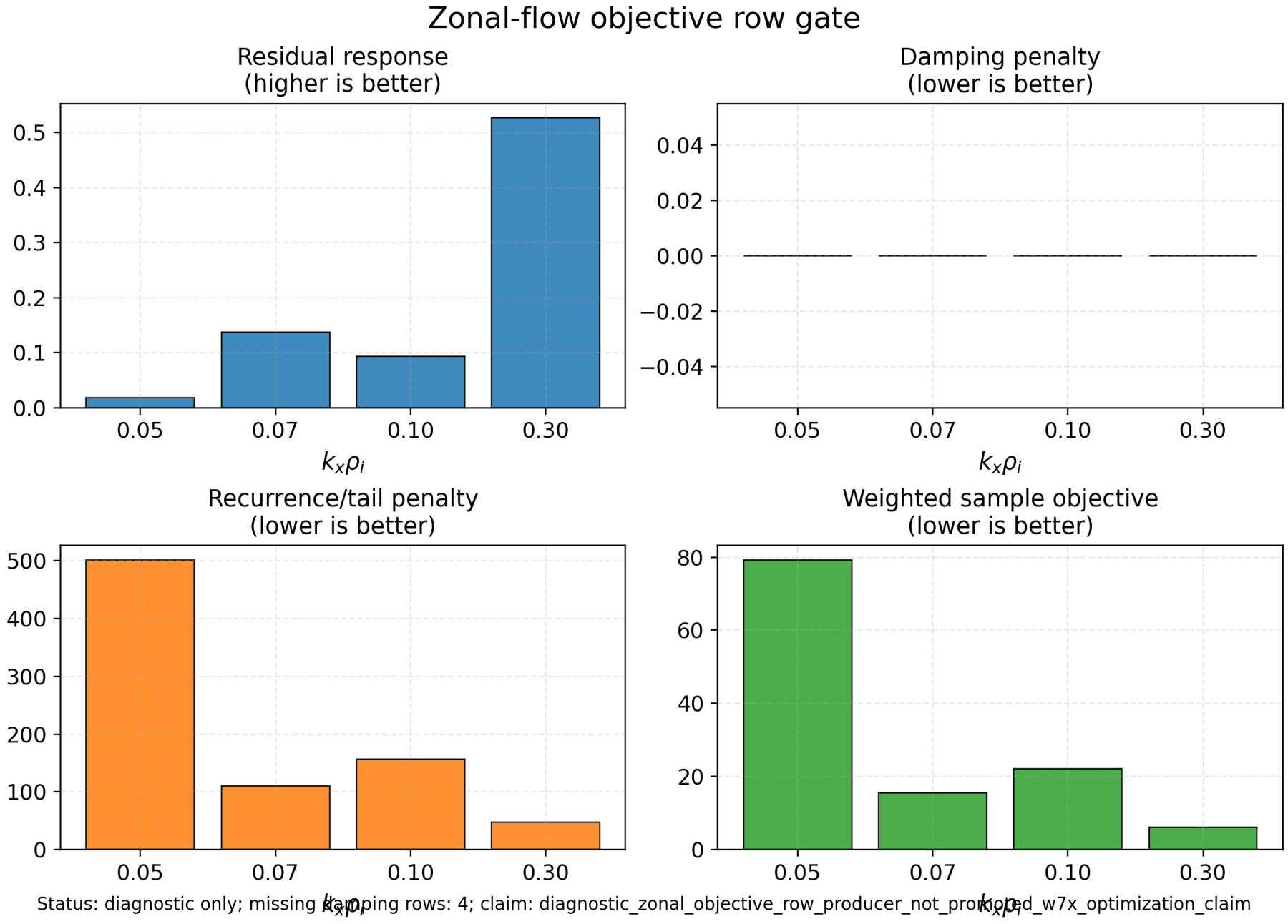
Zonal-flow objective row-production gate. The panel shows the row metrics consumed by the reduced objective for each W7-X k_x. Large residuals lower the inverse-residual penalty, while large late-window tail ratios remain explicit penalties. The current W7-X artifact is a diagnostic bridge, not a promoted optimization claim, because the damping fits are not closed under the paper-facing normalization.

Connection to Literature

The current implementation is closest in spirit to direct microstability optimization [Jorge24]: it makes a differentiable linear or quasilinear transport proxy available inside a stellarator objective. It also follows the lesson from nonlinear turbulence optimization [Kim24]: final heat-flux claims must be audited with nonlinear windows because linear and quasilinear proxies can fail when nonlinear saturation physics changes.

The next manuscript-level step is therefore not to promote this reduced model as an absolute flux predictor. The correct next step is to replace the reduced feature map with a parity-checked in-memory geometry pipeline and then audit the optimized shapes with converged nonlinear GKX runs.

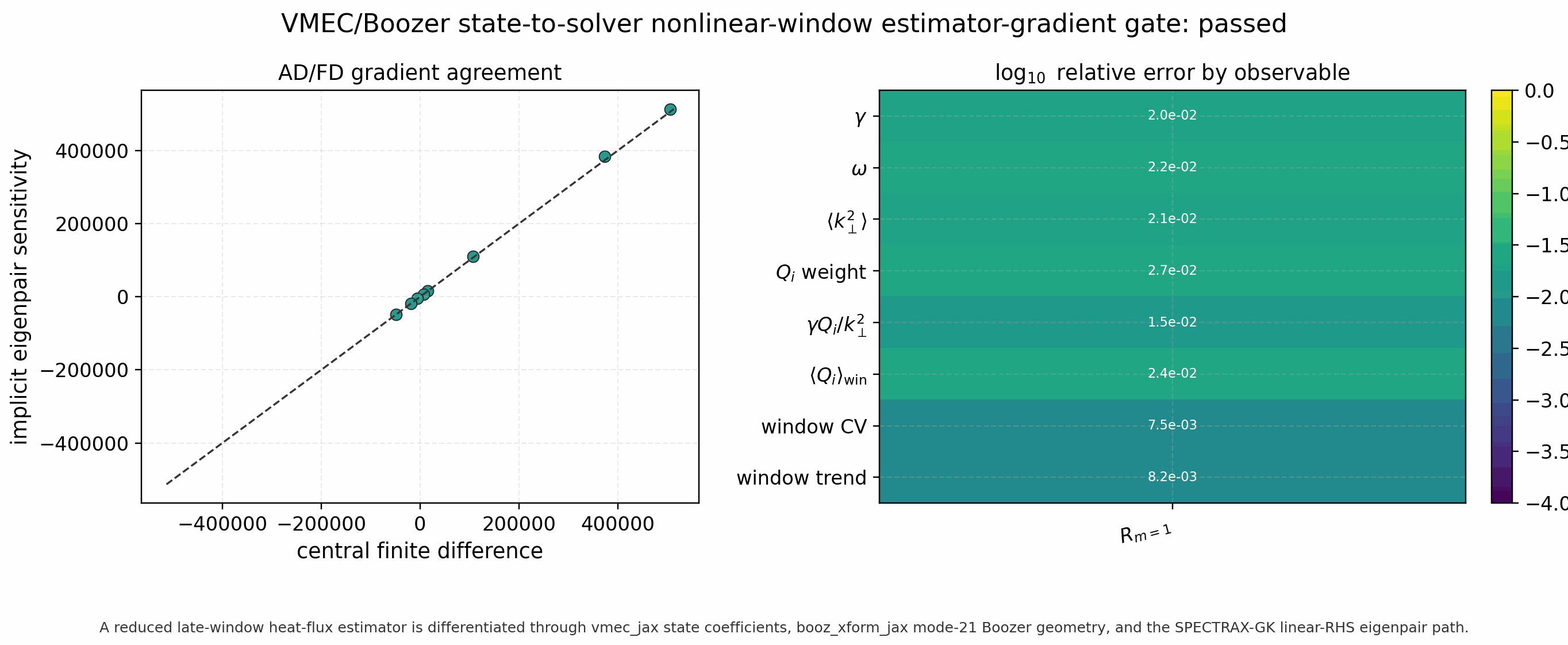
Solver-objective Geometry Gradients

The first production-adjacent solver-gradient gate now differentiates actual electrostatic linear-RHS eigenpair observables with respect to solver-ready geometry arrays. The gate uses the implicit left/right non-Hermitian eigenpair sensitivity system and compares the result against nearest-branch central finite differences for gamma, omega, <k_perp^2>, linear heat/particle-flux weights, and a mixing-length heat-flux proxy. This closes the FluxTubeGeometryData contract-level solver-gradient check and the first full vmex state-coefficient to booz_xform_jax to solver eigenfrequency-gradient gate. The companion QH all-surface artifact closes the reduced full-chain quasilinear heat-flux-weight gradient gate for the tracked manuscript fixture. A second Li383 low-resolution holdout now verifies the same frequency and quasilinear gradient contracts at mboz=nboz=21; the combined holdout matrix has maximum relative AD/finite-difference mismatch 4.9e-3 across the reduced linear/quasilinear objectives. Companion QH and Li383 reduced nonlinear-window estimator gates now differentiate a smooth late-window heat-flux envelope through the same VMEC/Boozer state path; the expanded matrix including those estimator rows has maximum relative mismatch 2.7e-2. This closes a multi-equilibrium bounded estimator-gradient check for nonlinear-window-style reduced objectives, but it does not close converged nonlinear-window turbulence gradients or broad optimized-equilibrium nonlinear transport claims.

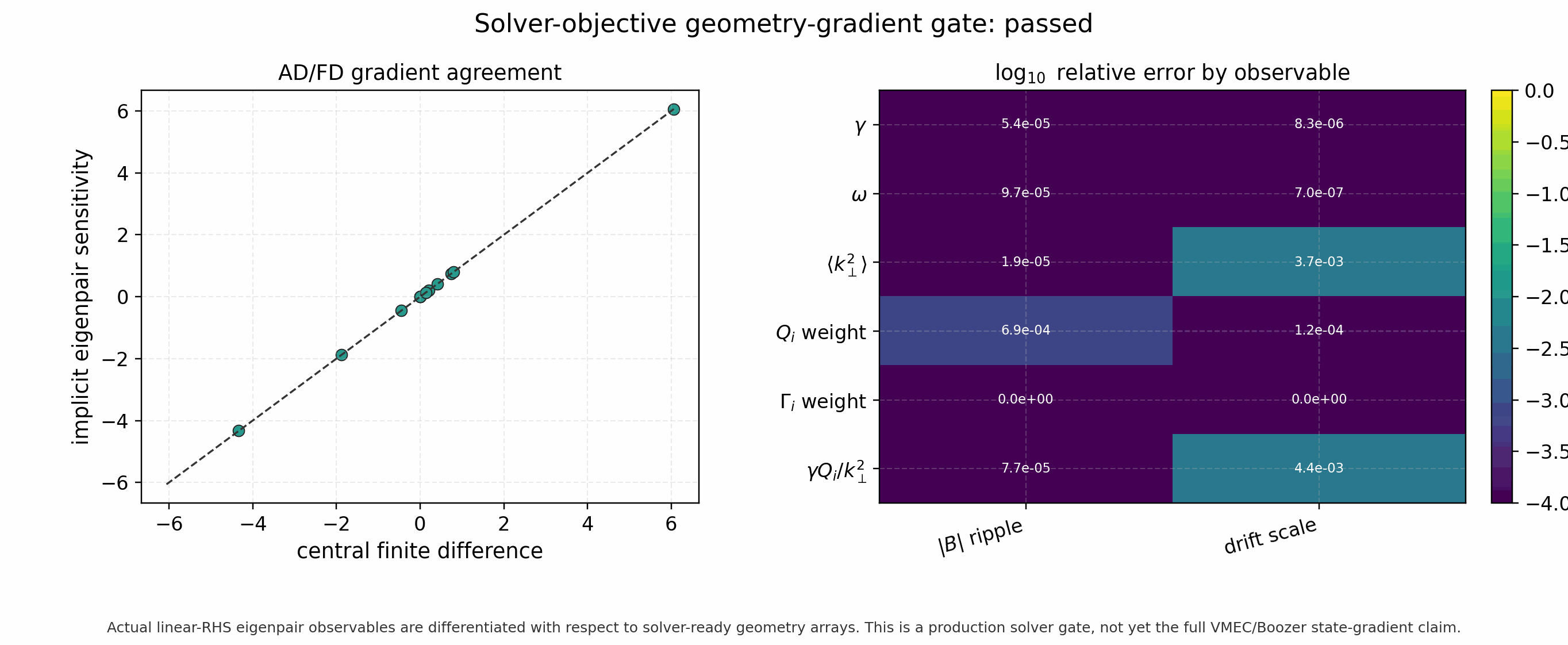
Solver-ready geometry-gradient gate. The left panel compares implicit eigenpair sensitivities with central finite differences; the right panel shows per-observable relative errors for the two geometry controls.

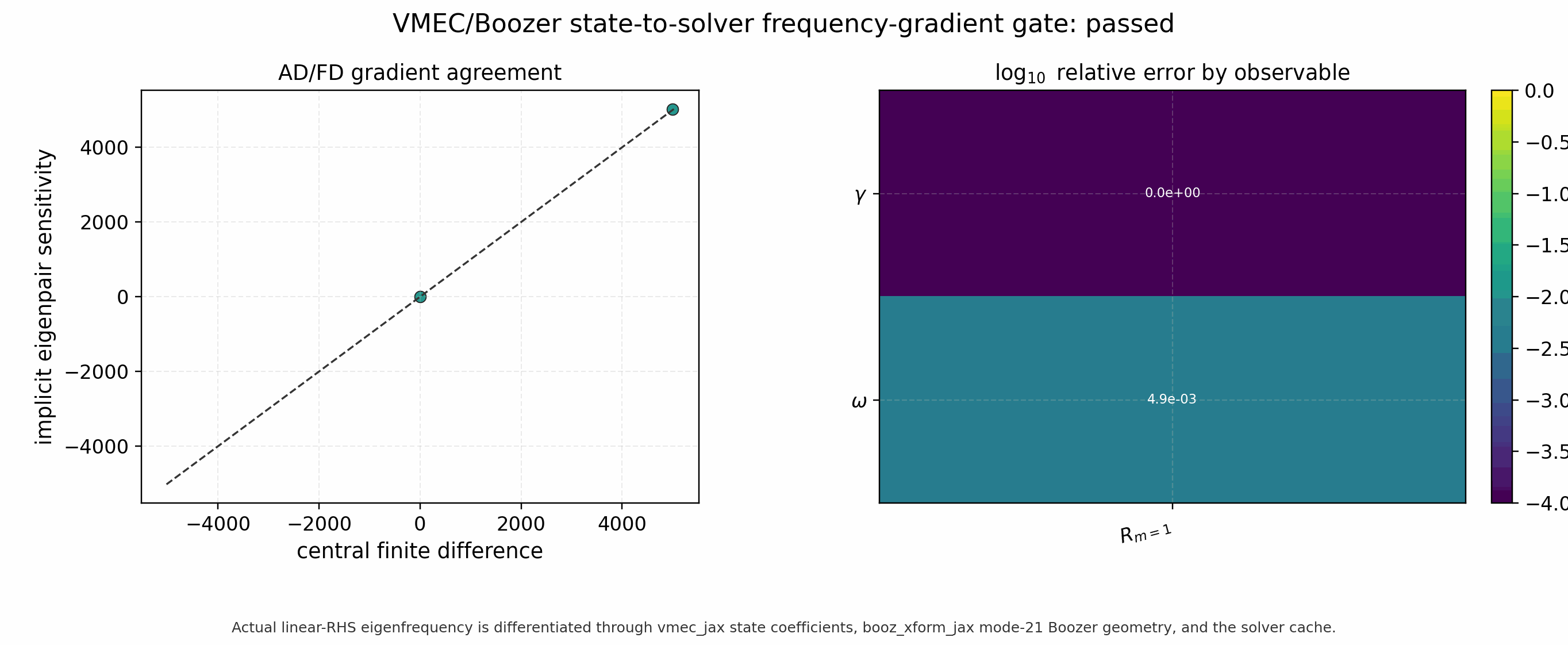
Full-chain VMEC/Boozer eigenfrequency-gradient gate. A real vmex state coefficient is perturbed, converted through booz_xform_jax with mboz=nboz=21, mapped into the GKX linear solver, and checked against central finite differences. The artifact tools also accept explicit VMEC radial_index, mode_index, and surface_index controls so conditioning scans can choose physically meaningful state perturbations without changing source code.

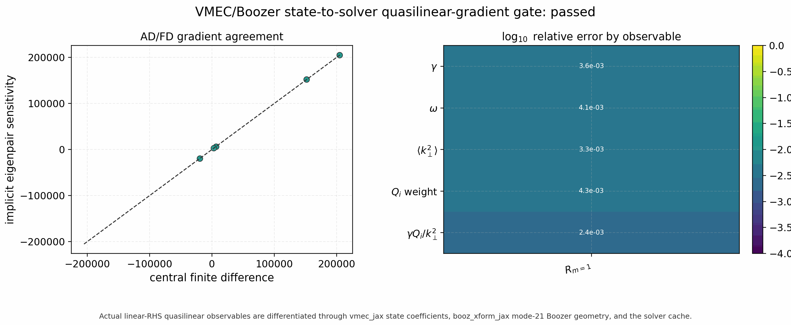
Full-chain VMEC/Boozer quasilinear-gradient gate. The same state coefficient is mapped through vmex and booz_xform_jax with mboz=nboz=21 and a richer Nl=2, Nm=3 GKX moment basis. The implicit left/right eigenpair sensitivity of gamma, omega, <k_perp^2>, the electrostatic heat-flux weight, and gamma Q_i/k_perp^2 agrees with central finite differences to 4.3e-3 relative error in the tracked artifact. This closes the linear/quasilinear full-chain gradient gate for reduced stellarator objectives on the all-surface QH fixture. The optional Boozer surface-stencil path is a memory-bounded diagnostic for larger equilibria, not the published accuracy gate; QI/QA multi-equilibrium transport-gradient promotion remains open until all-surface or otherwise accuracy-equivalent gates pass. This is still not a nonlinear-window heat-flux gradient claim.

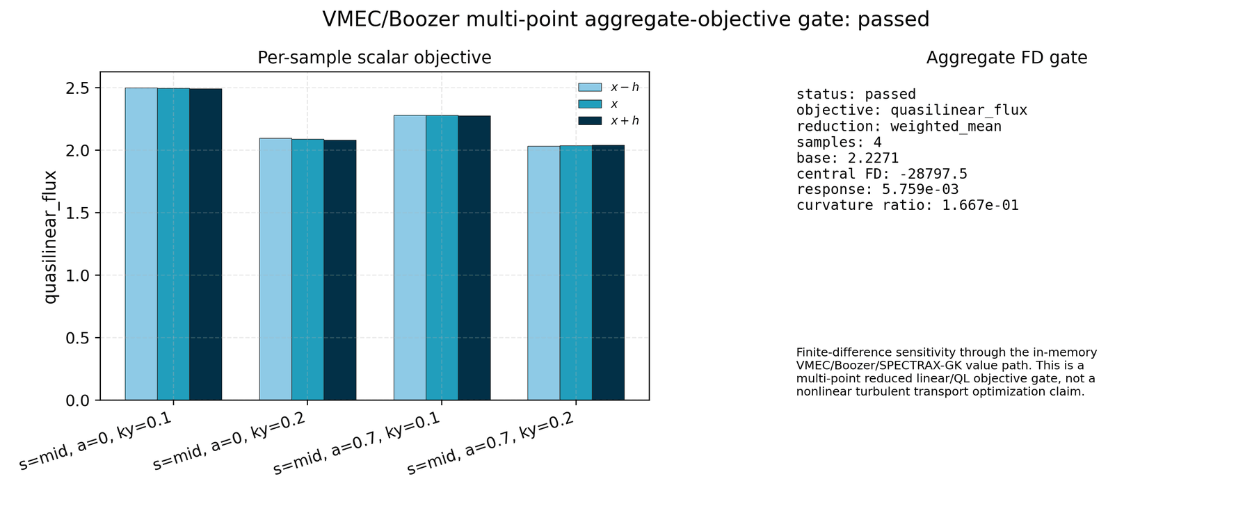
Multi-point VMEC/Boozer aggregate-objective gate. The tracked QH fixture evaluates the quasilinear proxy at two resolved k_y samples using mboz=nboz=21 and records the aggregate finite-difference response through the same in-memory VMEC/Boozer/GKX value path. This closes the software and artifact path for multi-k_y reduced objectives; it is not a nonlinear turbulent heat-flux optimization claim. The tracked two-k_y artifact intentionally does not satisfy the held-out surface/field-line promotion gate by itself.

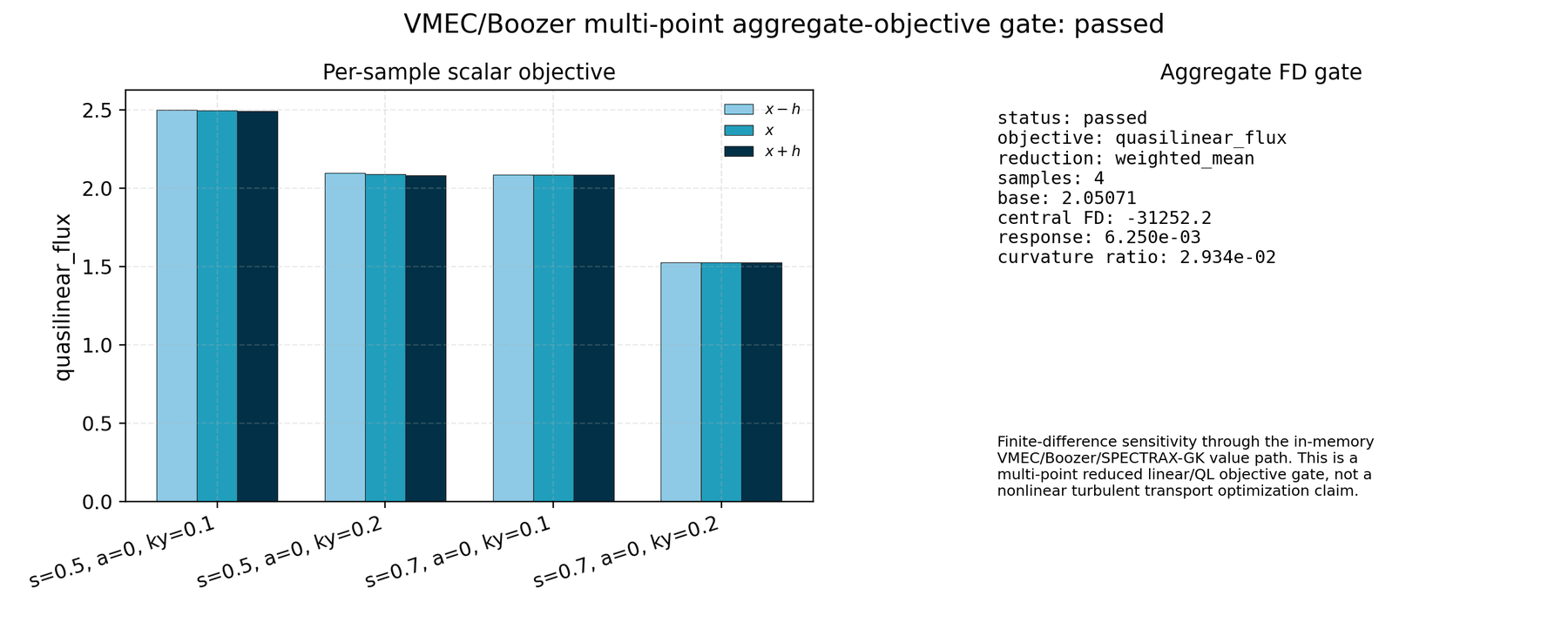
Physical-surface VMEC/Boozer aggregate-objective gate. The same QH fixture evaluates the quasilinear proxy at two normalized toroidal-flux values (torflux = 0.5 and 0.7) and two physical k_y rho_i values (0.1 and 0.2). The JSON/CSV sidecars record the requested physical torflux and k_y values, the resolved solver selected_ky_index, and ky_abs_error. The companion vmec_boozer_torflux_reduced_portfolio_guard.json passes with two surfaces, one field line, and two k_y samples; this is surface-axis reduced-objective evidence, not nonlinear turbulent-transport optimization evidence.

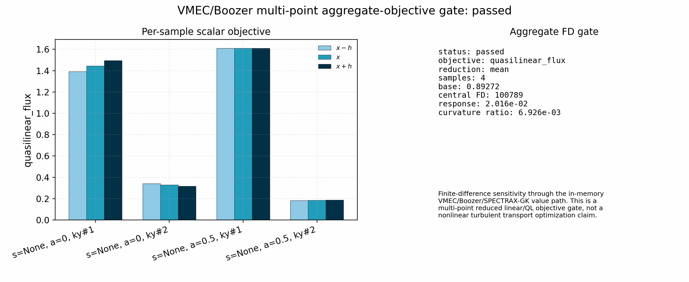
Multi-alpha VMEC/Boozer aggregate-objective gate. The QH fixture repeats the same quasilinear finite-difference audit over two field lines (alpha = 0 and 0.5) and two k_y samples using mboz=nboz=21. The tracked artifact has four samples, passes the curvature gate with curvature ratio about 6.9e-3, and is the current reduced-objective evidence for field-line coverage. It still remains a reduced linear/quasilinear objective gate, not an optimized-equilibrium nonlinear transport claim. The reduced-portfolio guard in docs/_static/vmec_boozer_reduced_portfolio_guard.json now verifies that these real rows satisfy the backend-free reducer contract and the growth/QL AD/FD provenance boundary.

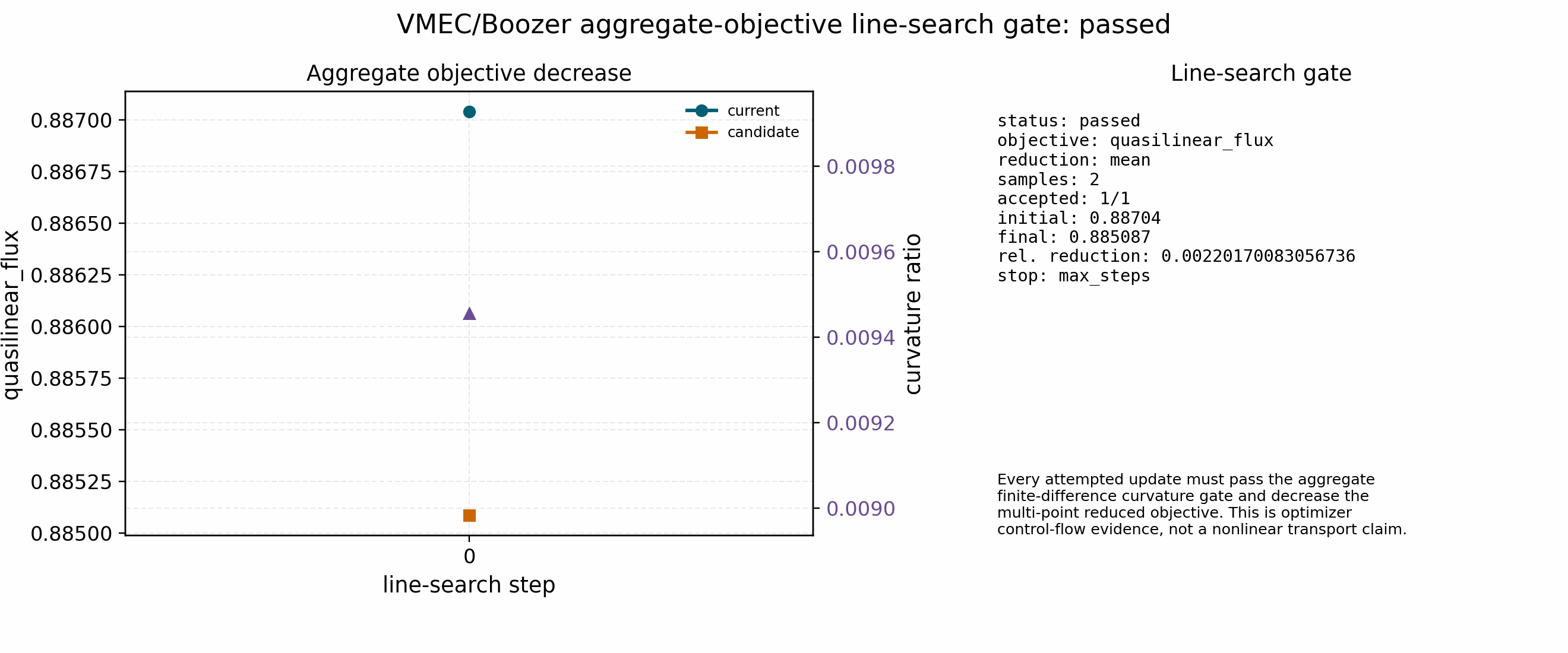
Multi-point VMEC/Boozer aggregate-objective line-search gate. The tracked QH fixture applies one curvature-gated VMEC coefficient update to the two-k_y quasilinear proxy aggregate and accepts it only because the candidate decreases the objective while the finite-difference gate remains conditioned. This is optimizer control-flow evidence for reduced objectives, not a nonlinear turbulent transport optimization claim. It must be paired with held-out surface_index or field-line alpha validation before it can support an optimized-equilibrium transport claim.

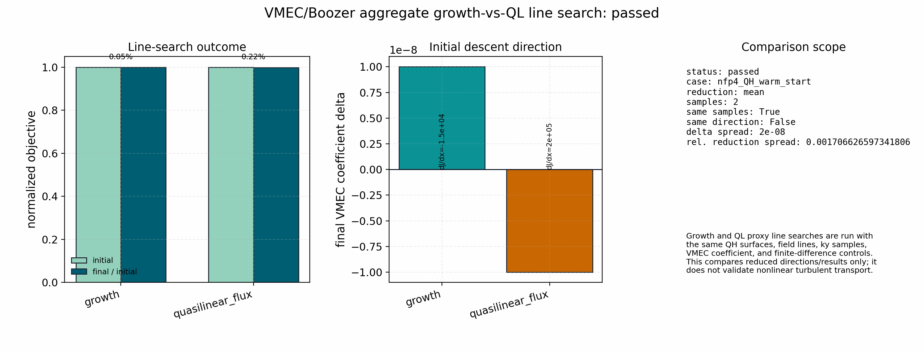
Growth-vs-quasilinear aggregate line-search comparison. The growth and quasilinear proxy objectives both pass a one-step curvature-gated line search on the same QH sample set, but their initial descent directions differ. This is important for manuscript claims: optimizing growth rate, quasilinear proxy, and nonlinear transport are related but not identical objective choices, so each must carry its own validation and holdout gate.

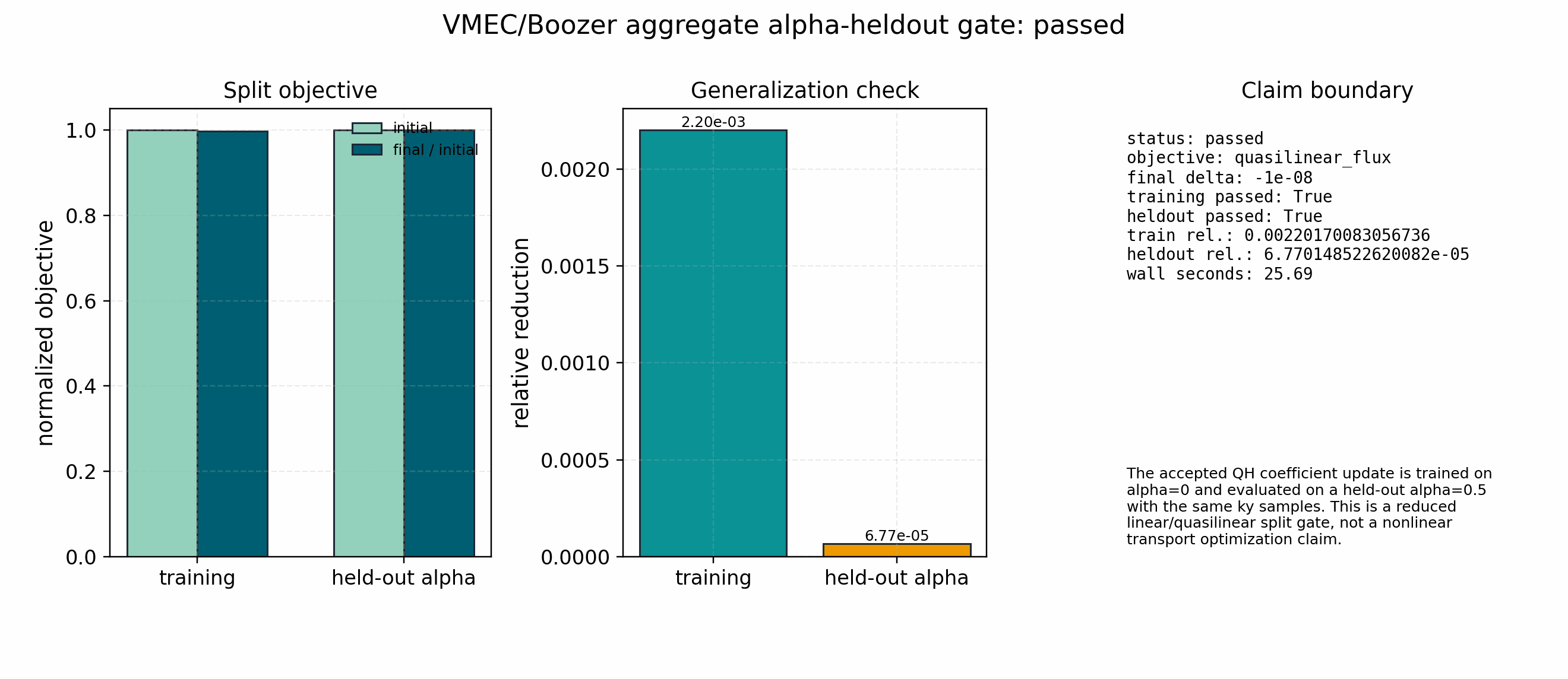
Alpha-heldout aggregate line-search gate. The same accepted quasilinear update is trained on the alpha=0 QH field line and evaluated on the held-out alpha=0.5 field line with the same two k_y samples. The tracked artifact passes, with training relative reduction about 2.2e-3 and held-out relative reduction about 6.8e-5. This is useful reduced field-line generalization evidence, but it is intentionally blocked from the production promotion gate because it is still a reduced linear/quasilinear objective split, not a nonlinear transport validation.

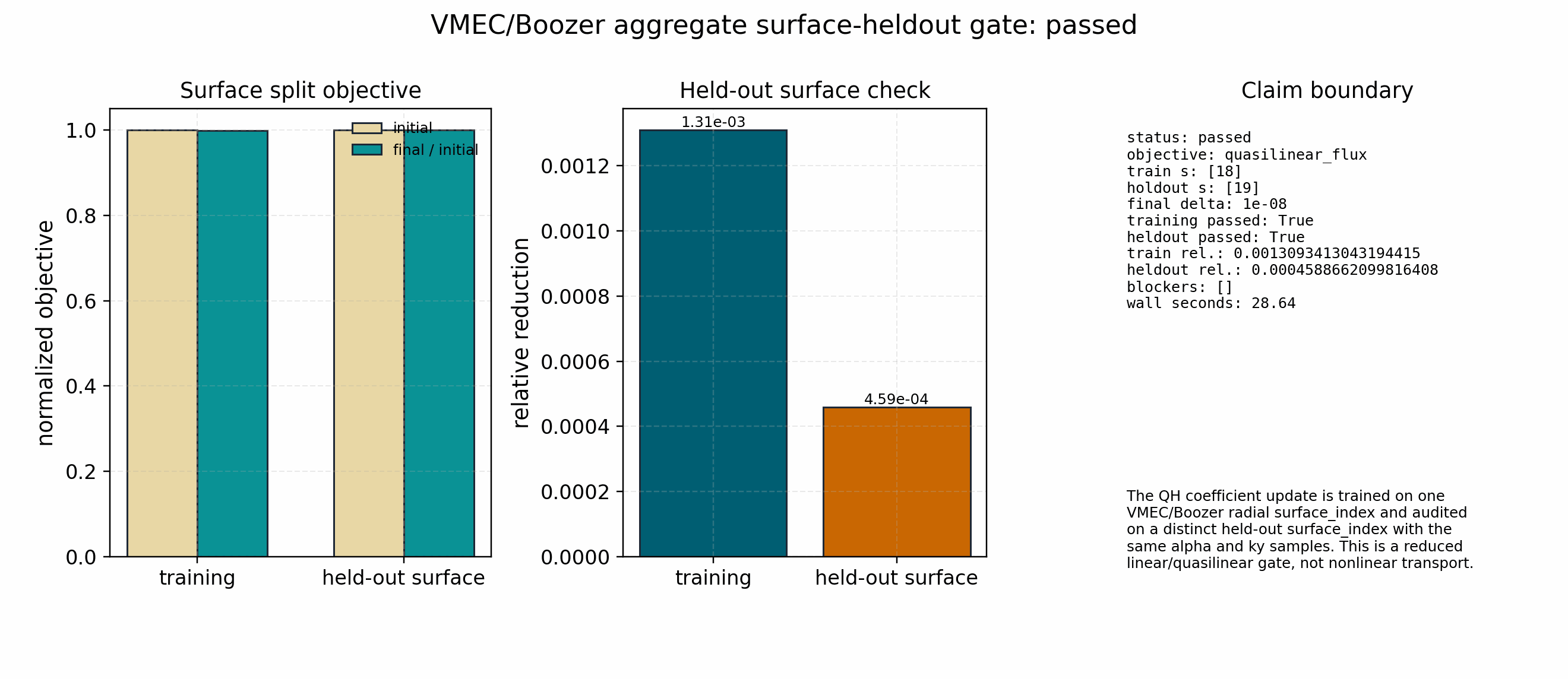
Surface-heldout aggregate line-search gate. The QH quasilinear update is trained on explicit surface_index = 18 and evaluated on held-out surface_index = 19 with the same alpha=0 and two k_y samples. The tracked artifact passes with training relative reduction about 1.31e-3 and held-out-surface relative reduction about 4.59e-4. This closes a true reduced surface-generalization check; it still remains a reduced linear/quasilinear objective gate rather than a nonlinear transport validation.

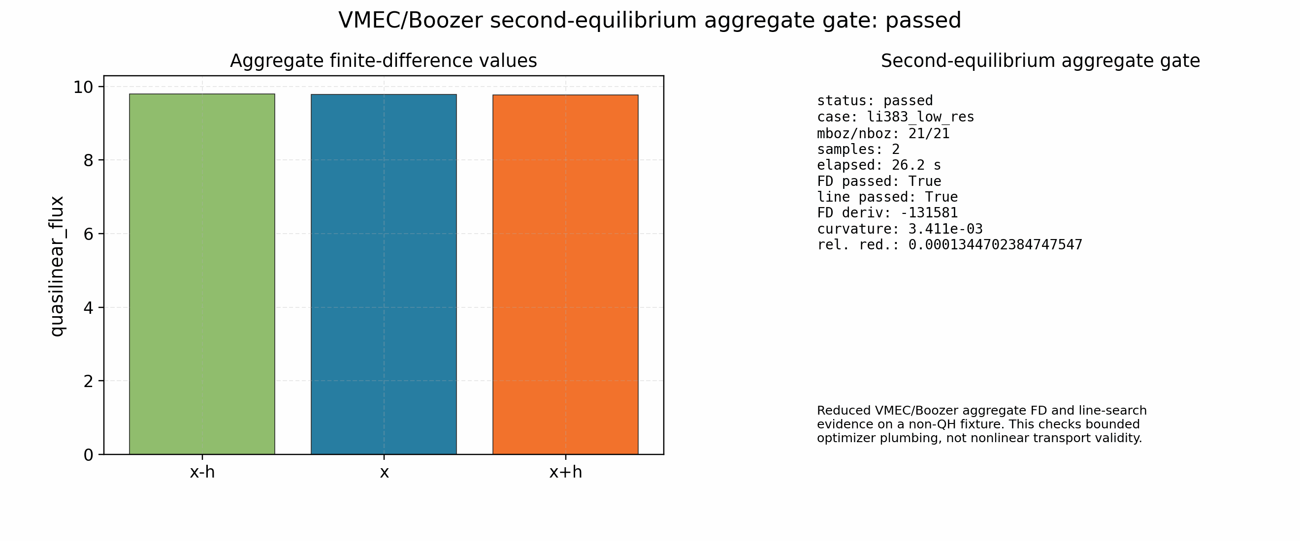
Second-equilibrium aggregate-objective gate. The Li383 fixture passes the same mode-21 VMEC/Boozer aggregate finite-difference and one-step line-search path with two k_y samples. The finite-difference curvature ratio is about 3.4e-3 and the line search reduces the reduced quasilinear objective by about 1.34e-4. This is second-equilibrium optimizer-plumbing evidence, not a calibrated saturated-flux or nonlinear transport claim.

Reduced nonlinear-window estimator-gradient gate for the QH fixture. The full VMEC/Boozer state-to-solver path produces linear-RHS observables, then a smooth RK2 late-window envelope maps those observables to mean heat flux, window coefficient of variation, and normalized trend. The plot compares implicit eigenpair AD sensitivities against central finite differences. The companion Li383 artifact is included in the holdout matrix. These are differentiability and conditioning gates for reduced objectives, not converged nonlinear-turbulence heat-flux-gradient claims.

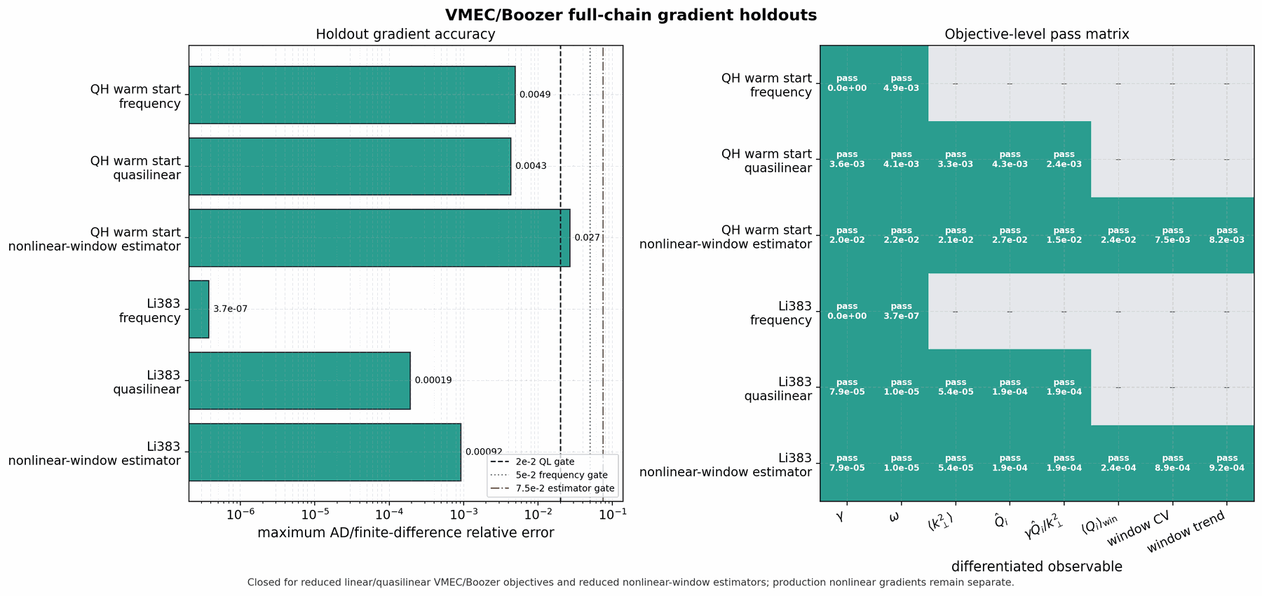
Multi-equilibrium VMEC/Boozer gradient holdout matrix. QH and Li383 frequency, quasilinear, and reduced nonlinear-window estimator gates all pass with mboz=nboz=21. The matrix is a reduced differentiability gate; converged nonlinear-window turbulence gradients remain a separate promotion requirement.

Promotion Gates for Full VMEC/Boozer/GK Optimization

The full production stellarator optimization claim remains open until all of the following pass:

1. vmex state to booz_xform_jax to FluxTubeGeometryData works in memory without writing intermediate VMEC or EIK files. The current bridge already validates the optional vmex boundary derivative, real vmex metric-tensor derivatives, a real non-axisymmetric VMEC field-line tensor derivative through vmex.geom plus vmex.vmec_bcovar, a real VMEC tensor-derived flux-tube mapping derivative, a real booz_xform_jax spectral derivative, and a bounded Boozer-|B|-to-flux-tube mapping derivative. It now also starts from a real vmex VMECState, perturbs VMEC Fourier coefficients, converts through booz_xform_jax, and checks GKX field-line geometry-observable derivatives against central finite differences. The same artifact now records a direct-VMEC-tensor vs imported-VMEC/EIK array-parity audit plus a Boozer equal-arc core audit. The core audit now matches the imported bmag, bgrad, gradpar, q, s_hat, Jacobian, zero-beta gds*/grho metric convention, and zero-beta loaded cvdrift/gbdrift drift convention at release tolerance. The remaining gap is finite-beta and broader production-runtime drift parity beyond the tracked zero-beta equal-arc fixtures before broad transport-gradient claims are promoted. The reverse-mode state-level bridge additionally requires booz_xform_jax at or after commit 1d5e8c; earlier JAX Boozer transforms can have finite values but non-finite zero-mode cotangents.

2. The sampled field-line arrays match the existing imported-VMEC/EIK runtime path for at least one small equilibrium.

3. Geometry-observable gradients match central finite differences for the in-memory bridge.

4. Linear growth-rate, frequency, and quasilinear-weight gradients through the solver-ready geometry contract pass finite-difference or implicit-eigenpair checks. This is closed by docs/_static/solver_objective_gradient_gate.json for a small actual linear-RHS fixture. The full mode-21 VMEC/Boozer state-to-solver eigenfrequency gate is also closed by docs/_static/vmec_boozer_solver_frequency_gradient_gate.json. The full mode-21 VMEC/Boozer state-to-solver quasilinear heat-flux-weight gate is closed by docs/_static/vmec_boozer_quasilinear_gradient_gate.json on the tracked all-surface QH fixture. The multi-equilibrium reduced linear/quasilinear and nonlinear-window estimator holdout gate is closed by docs/_static/vmec_boozer_gradient_holdout_matrix.json for QH and Li383 at mboz=nboz=21. The finite-beta shaped-pressure eigenfrequency-gradient gate is closed separately by docs/_static/vmec_boozer_shaped_pressure_solver_frequency_gradient_gate.json with max relative AD/finite-difference error about 6.4e-11. The finite-beta shaped-pressure quasilinear-gradient gate is closed by docs/_static/vmec_boozer_shaped_pressure_quasilinear_gradient_gate.json with max relative error about 2.1e-4. The finite-beta shaped-pressure reduced nonlinear-window estimator-gradient gate is closed by docs/_static/vmec_boozer_shaped_pressure_nonlinear_window_gradient_gate.json with max relative error about 2.1e-4; this still does not promote finite-beta converged nonlinear transport gradients. Larger QI/QA nonlinear-window transport holdouts are still promotion work: QI is currently conditioning-limited when forced through the narrow diagnostic stencil, while the QA low-resolution all-surface Boozer transform exceeds the available office GPU memory at mboz=nboz=21.

5. Host scalar materialization in production runtime caches is removed or isolated so geometry parameters remain traceable.

6. A nonlinear heat-flux objective has a validated adjoint, VJP, or robust stochastic/finite-difference estimator with a documented window rule. The reduced estimator-gradient gate at docs/_static/vmec_boozer_nonlinear_window_gradient_gate.json and the Li383 holdout at docs/_static/vmec_boozer_li383_nonlinear_window_gradient_gate.json cover the first multi-equilibrium bounded estimator path; production claims still need converged nonlinear-window turbulence gradients or robust optimized-equilibrium finite-difference audits.

7. Optimized geometries pass multi-field-line, multi-surface, grid/window convergence, and nonlinear holdout gates before being used for transport claims. The current multi-point VMEC/Boozer aggregate API closes the software plumbing for this gate, but the manuscript claim remains bounded until the corresponding aggregate artifacts pass on the selected equilibria. tools/release/check_vmec_boozer_gates.py aggregate-holdout is the artifact-level promotion check for this boundary: aggregate finite-difference and line-search artifacts must pass on the same training sample set, and at least one independent passed validation artifact must cover a held-out surface_index or field-line alpha. Additional k_y coverage is useful, but k_y-only holdout evidence does not satisfy the surface/field-line gate. A passed replicated nonlinear-window ensemble is also required before the optimized-equilibrium claim can be promoted from reduced-objective evidence to production nonlinear transport evidence. The current frozen promotion artifact, docs/_static/vmec_boozer_aggregate_holdout_promotion_gate.json, is blocked as intended: reduced held-out-alpha and held-out-surface artifacts now pass, but they remain reduced-objective evidence, while the D-shaped and circular replicated nonlinear-window ensembles are holdout/calibration evidence. The selected optimized QA equilibrium now has its own replicated long-window nonlinear audit, which closes the optimized-equilibrium post-transient transport-window evidence requirement for this scoped candidate. The current selected candidate has completed the release n64 nonlinear transport replicate ladder over t=250,350,450,700 continuations with two random-seed replicates and one timestep replicate. The t=[350,700] ensemble passes finite-flux, running-window, block/SEM, replicate-spread, and optimized-equilibrium marker gates, with ensemble mean ion heat flux 10.19, mean-relative spread 0.038, and combined SEM/mean 0.021.

   The current QA vmex optimized-equilibrium candidate has also been screened through the GKX linear/quasilinear runtime before launching the large nonlinear campaign. On the sampled ITG branch k_y rho_i = 0.095, 0.190, 0.300, 0.476, 0.667, all fitted growth rates are negative, with the least damped point at gamma≈-0.015. The quasilinear mixing-length diagnostic therefore reports zero saturated heat flux because stable modes are excluded by the current growth-floor rule. The nonlinear audit for this candidate is therefore interpreted as a post-transient optimized-equilibrium transport-window check, not as evidence that the uncalibrated quasilinear zero-flux estimate predicts an absolute saturated flux. The separate projected-gradient candidate above is a negative long-window transfer audit and is intentionally not used as the selected optimized-equilibrium success case.

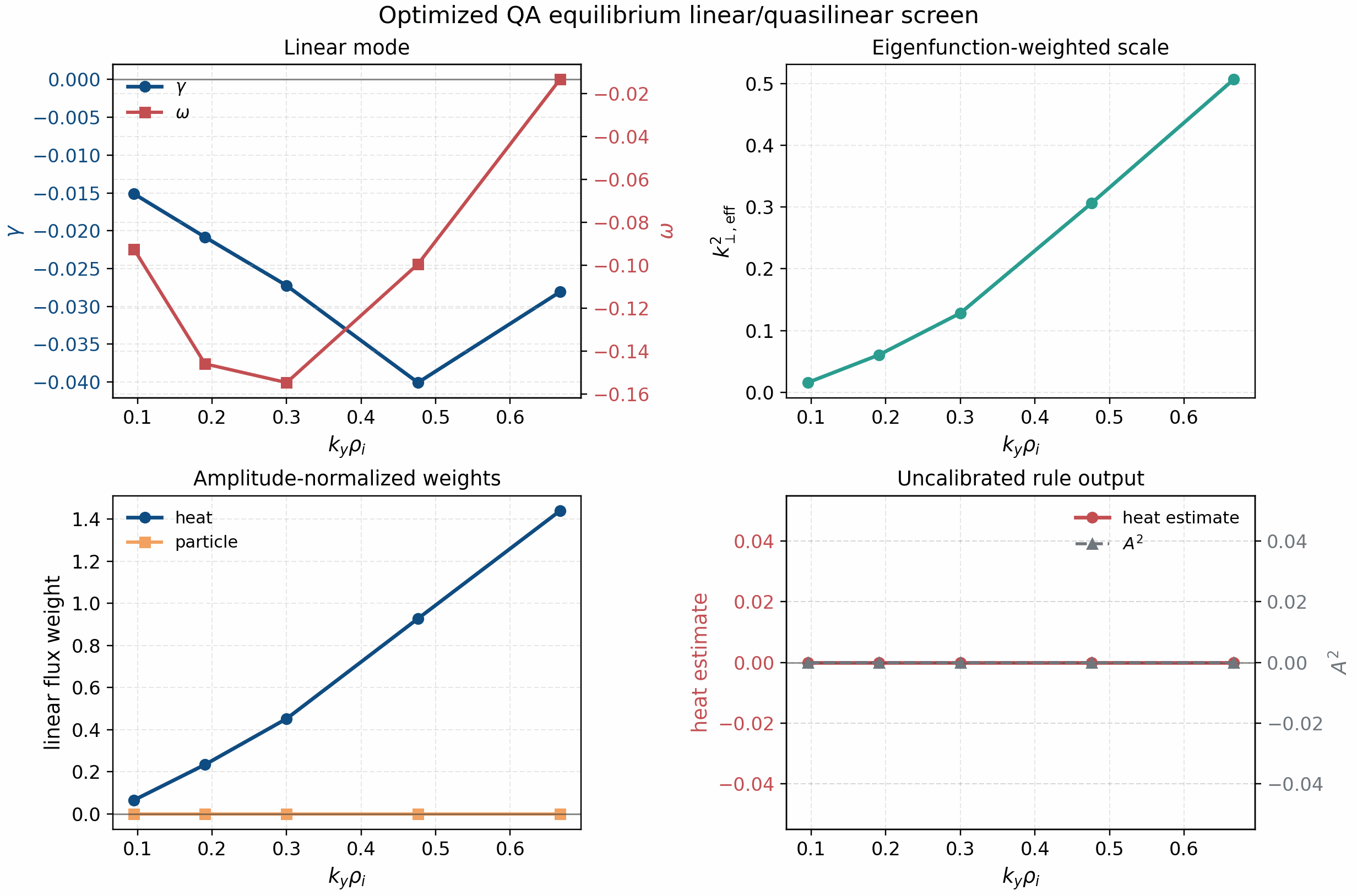
Linear/quasilinear screen for the QA optimized-equilibrium candidate from vmex. The sampled ITG branch is linearly damped across the scan, so the uncalibrated quasilinear heat-flux estimate is zero under the stable-mode exclusion rule. The subsequent nonlinear audit shows finite post-transient heat flux, so this panel should be read as a stability/branch screen rather than as an absolute-flux prediction.

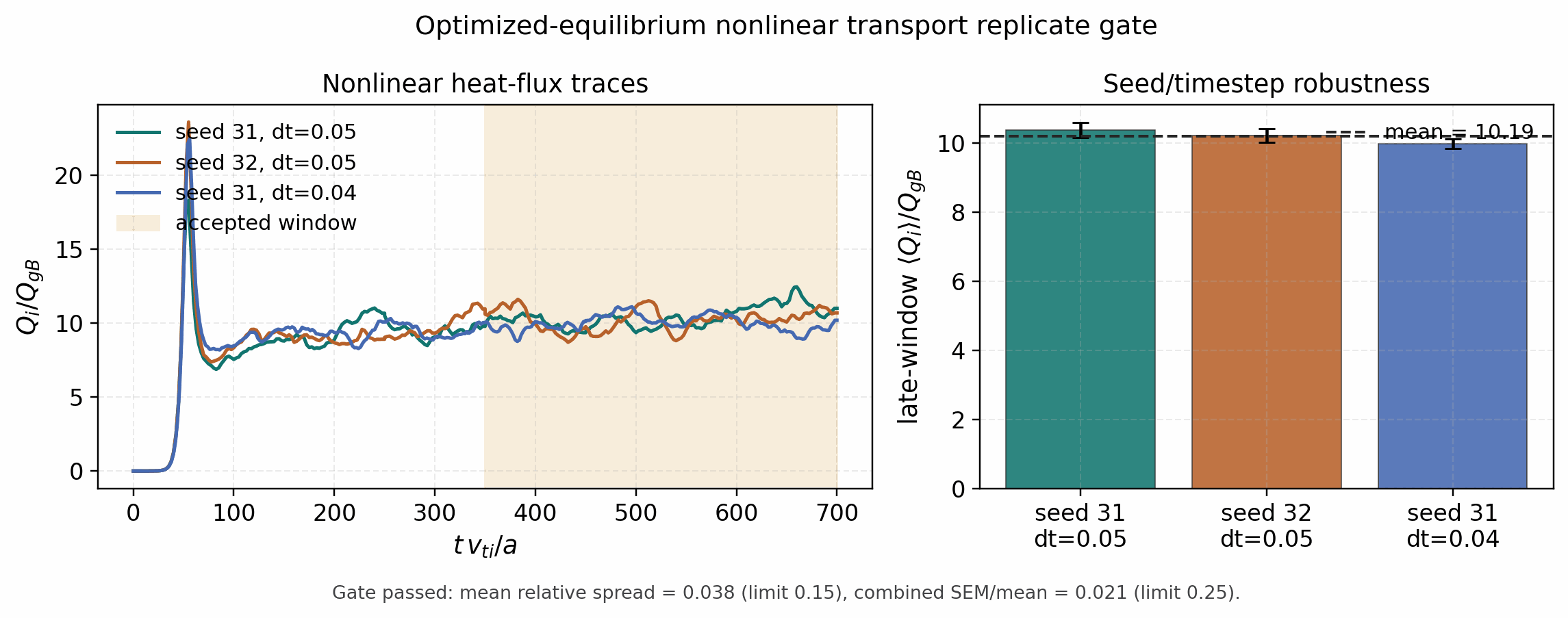
Optimized-equilibrium nonlinear replicate gate. Two seed replicates and one timestep replicate are advanced to t≈700 at n64 and accepted over the post-transient window t=[350,700]. The ensemble passes with mean ion heat flux 10.19, mean-relative spread 0.038, and combined SEM/mean 0.021. This closes the scoped optimized-equilibrium transport-window evidence gate; broader nonlinear turbulence-gradient and absolute-flux model claims remain separate gates.

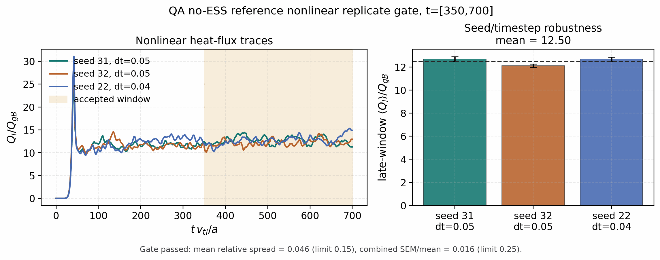
Matched no-ESS reference replicate gate. The valid finite-transform QA no_ess equilibrium from the same vmex campaign is advanced with the same grid, seeds, timestep variant, and post-transient window as the selected optimized QA/ESS equilibrium. The reference ensemble passes with mean ion heat flux 12.50, mean-relative spread 0.046, and combined SEM/mean 0.016.

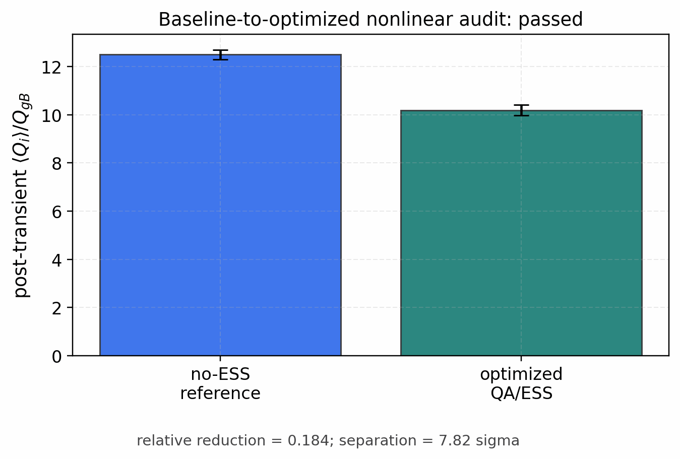
Matched baseline-to-optimized nonlinear audit. Against the validated no-ESS reference ensemble, the optimized QA/ESS equilibrium reduces the post-transient ion heat flux from 12.50 to 10.19. The relative reduction is 0.184 and the difference is separated by 7.82 combined SEMs. The zero-transform raw wout_initial.nc from the VMEC optimization is intentionally excluded because it cannot define the same finite-twist flux-tube baseline.

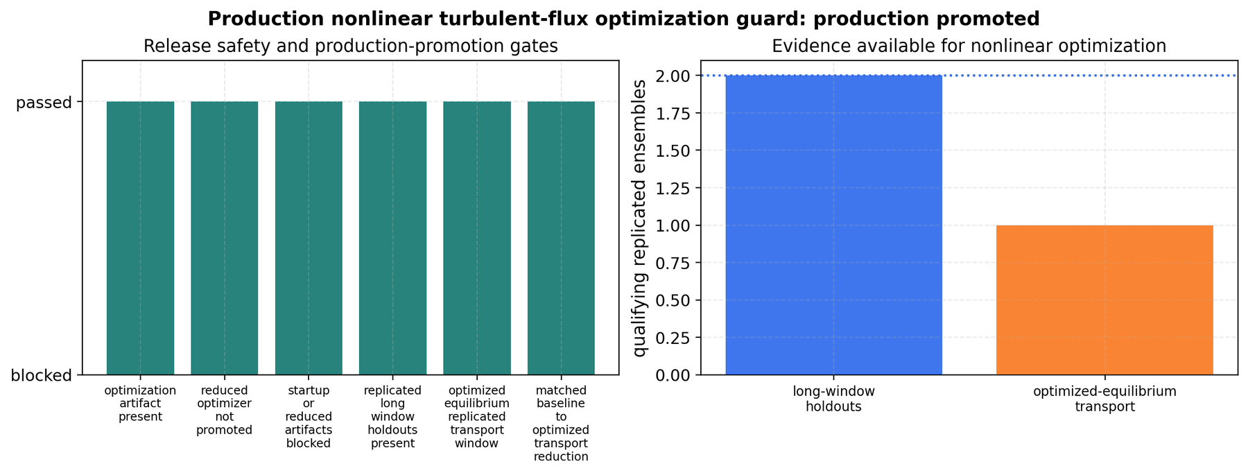
Production nonlinear turbulent-flux optimization guard. The release-safety side passes because startup and reduced nonlinear artifacts are explicitly blocked from production promotion and three long post-transient replicated holdout ensembles pass: D-shaped VMEC, circular VMEC, and the QH VMEC/Boozer held-out surface/field-line transport run. The selected optimized-equilibrium audit contributes one accepted matched audit, and the strict t=1500 growth/QL/nonlinear-window optimized-candidate traces close the optimized-equilibrium ensemble-count requirement. The current guard now promotes the scoped nonlinear turbulent-flux optimization evidence because 3/3 required matched audits pass the explicit 2% long-window reduction policy: the no-ESS-to-optimized QA/ESS audit gives 18.4%, while two full max-mode-5 projected-weight audits give 2.68% and 3.35%. Three strict t=1500 QA objective candidates remain negative transfer evidence, so broad multi-surface, multi-field-line nonlinear transport-optimization claims still require separate gates.

The release claim is now: GKX has a tested differentiable stellarator ITG objective-reduction workflow, long-window nonlinear holdout evidence, and a scoped optimized-equilibrium replicated nonlinear transport audit with a matched finite-transform no-ESS reference comparison. It is still not a universal absolute-flux quasilinear model, a nonlinear turbulence-gradient optimizer, or a broad multi-surface stellarator transport-optimization claim.

The next nonlinear turbulence-gradient promotion is now encoded as a fail-closed evidence gate in docs/_static/nonlinear_turbulence_gradient_evidence_gap_report.json. That gate requires paired baseline, plus_delta, and minus_delta nonlinear campaigns around the same VMEC/profile parameter, the same seed/timestep replicate set for every parameter state, post-transient heat-flux averages, passed ensemble uncertainty gates for all three states, and a central finite-difference audit with bounded response, asymmetry, condition number, and gradient uncertainty. Existing standalone replicated transport windows remain necessary evidence but are not sufficient to claim a production nonlinear turbulence gradient. The current real boundary-gradient sweep starts from the optimized QA/ESS equilibrium, re-equilibrates each perturbed VMEC input with vmex, runs three seed/timestep nonlinear replicates to t=900 for each parameter state, and analyzes the common t=[450,900] transport window. The tracked ZBS(1,0) 5% campaign closes the earlier finite-difference locality blocker: fd_asymmetry_rel = 0.274 and the response fraction is 0.0685. It still fails closed because the propagated gradient uncertainty is 0.768 > 0.5. The companion ZBS(1,1) 5% campaign gives the complementary negative result: gradient_uncertainty_rel = 0.225 passes, but fd_asymmetry_rel = 0.663 is still above the locality gate. This is now a robust production-candidate audit set, not a promoted nonlinear turbulence-gradient validation. A later seed-5 follow-up of the best ZBS(1,0) bracket kept the baseline/plus/minus long-window ensembles valid but did not close the claim: gradient_uncertainty_rel increased to about 1.18, fd_asymmetry_rel was about 0.520, and one matched-seed central finite difference changed sign. The scientific conclusion is therefore fail-closed: the current single-control bracket is a useful diagnostic, but it is not efficient to keep adding replicas at the same amplitude without a new locality/amplitude sweep or a smoother composite profile-gradient direction.

docs/_static/nonlinear_turbulence_gradient_candidate_ranking.json summarizes the completed RBC(1,1), ZBS(1,1), and ZBS(1,0) audits. The controls fail in complementary ways: ZBS(1,1) is statistically clean but nonlocal, whereas ZBS(1,0) can be local but is too noisy. The tracked RBC(1,1) sweep shows finite-difference asymmetry increasing from about 0.897 to 1.895; a larger bracket is therefore not a defensible cure.

The full overdetermined QA/ESS audit completed 33 long-window outputs and promoted no control. Its best RBC(1,1) candidate remains above the relative gradient-uncertainty gate (0.683 > 0.5). The later 7.5% ZBS(1,0) bracket resolves the response and locality (response_fraction = 0.0319, fd_asymmetry_rel = 0.044) but fails the plus-state spread and propagated uncertainty criteria. These are retained as negative physics evidence, not as machinery for generating further plans.

The retained variance-reduction workflow uses matched control-mean pairs. Four initial matched pairs were insufficient, while the independent 21-pair campaign over t=[600,1100] passed its scoped combined-uncertainty gate. This validates the estimator for this specific bracket; it does not justify a broad nonlinear turbulent-flux optimization claim.

Because both single-control amplitude sweeps point away from more blind replicas, GKX now also targets a smoother multi-coefficient direction. The tracked docs/_static/qa_ess_descent_profile_direction_rel2_manifest.json uses the current long-window evidence signs to define a 2% descent-oriented direction: decrease ZBS(1,1) while increasing ZBS(1,0) and RBC(1,1) with smaller weights. The finite-difference scalar is the Euclidean norm of the actual coefficient-change vector, so a successful downstream audit would measure a directional sensitivity per boundary-coefficient norm. That full campaign has now been run with real re-equilibrated VMEC files and matched t=900, n64:64:64:40:40 seed/timestep replicates. The output gates pass for all nine runtime files, and the baseline and minus replicated ensembles pass, but the plus ensemble fails its spread gate. The resulting central finite-difference artifact remains fail-closed: response_fraction≈0.052 is resolved, but fd_asymmetry_rel≈1.37 and gradient_uncertainty_rel≈1.13 exceed the promotion gates. This is a useful negative production-candidate audit, not a promoted nonlinear turbulence-gradient claim.

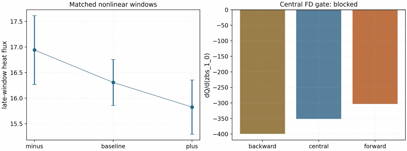
QA/ESS ZBS(1,0) 5% long-window nonlinear turbulence-gradient gate. The left panel shows the replicated t=[450,900] heat-flux means for minus, baseline, and plus states; the right panel compares backward, central, and forward finite-difference gradients. The artifact is a production-candidate long-window campaign, but it remains blocked because the propagated gradient uncertainty is still above the release gate.

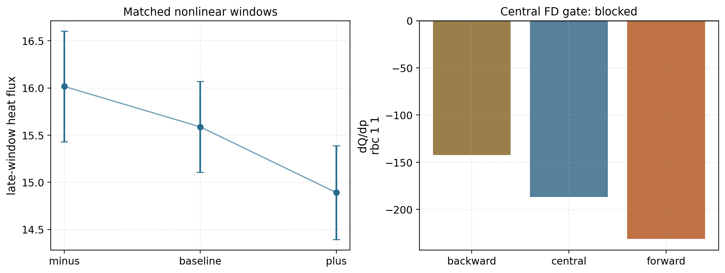
QA/ESS overdetermined RBC(1,1) 3% long-window nonlinear-gradient gate. This remains the best completed overdetermined candidate after the targeted seed33/seed34 follow-up: all five-member state ensembles pass and the backward/forward finite-difference asymmetry is below the locality gate. The artifact still fails closed because propagated uncertainty remains above the production threshold, so it supports model-development and next-campaign design rather than a promoted nonlinear turbulence-gradient claim.

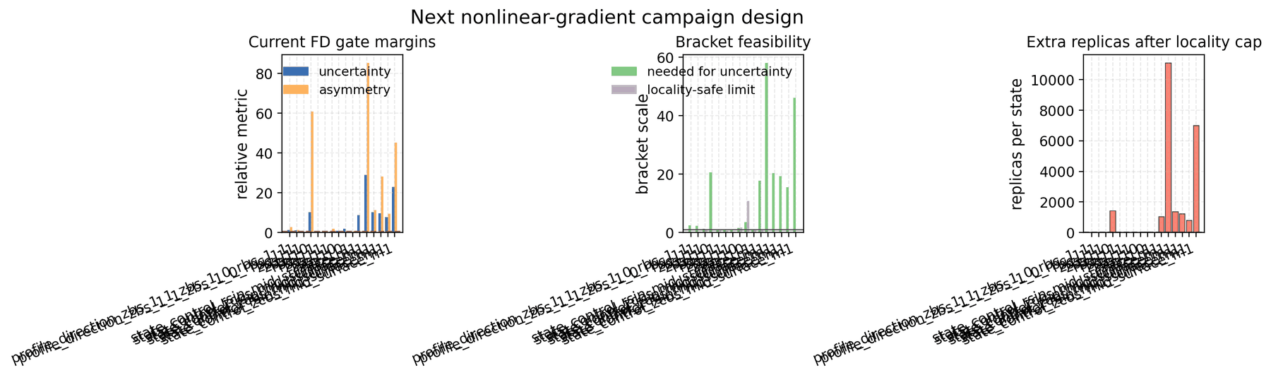
Next nonlinear-gradient campaign design gate. The left panel shows the current uncertainty and asymmetry margins, the middle panel compares the bracket scale required by uncertainty to the locality-safe bracket scale, and the right panel estimates extra replicas per state after applying the locality cap. The refreshed artifact now scans all 16 tracked central-FD gates: no candidate is promoted, one legacy candidate admits a bounded matched-replica follow-up, and the remaining 15 candidates require replacement, locality repair, or variance reduction before more long-window GPU time is justified. The top-level action is now to attack the plus-state variance limiter with paired-seed or control-variate design.

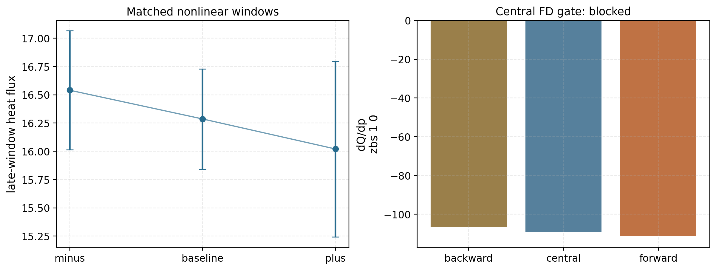
QA/ESS ZBS(1,0) 7.5% bounded nonlinear-gradient follow-up. The response and finite-difference locality gates now pass, but the plus-state replicated window is too broad and the propagated gradient uncertainty is too large. This artifact should be read as fail-closed evidence motivating variance reduction or a better-conditioned observable, not as a promoted nonlinear turbulence-gradient.

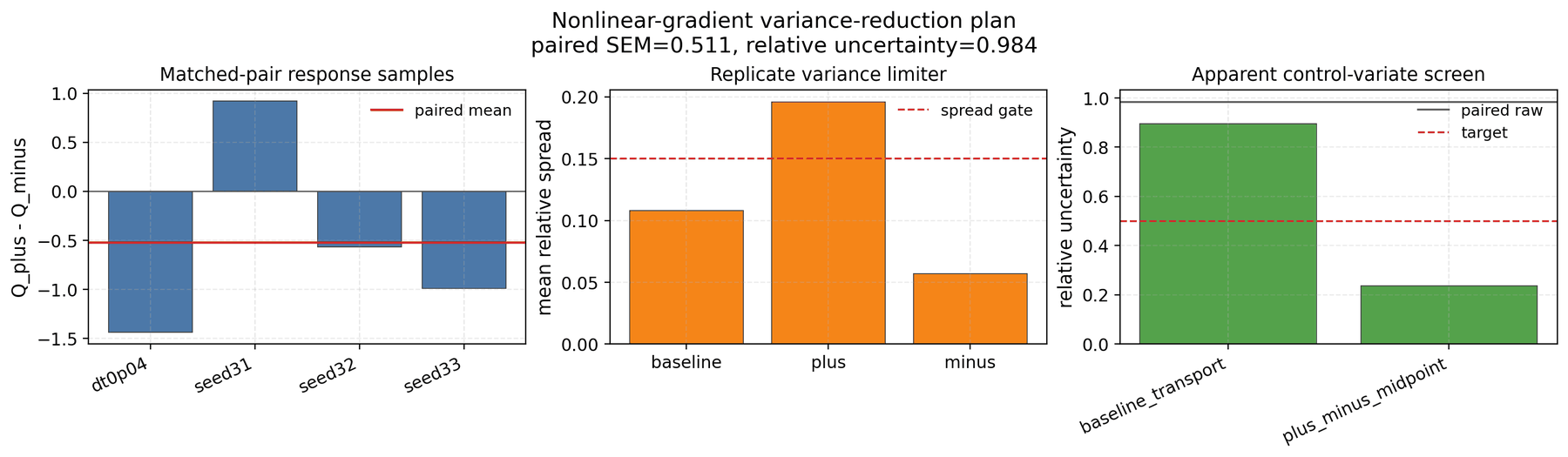
QA/ESS ZBS(1,0) rel7.5 paired-seed variance-reduction plan. The left panel shows matched plus-minus response samples for common seed/timestep labels; the middle panel identifies the plus state as the replicated-window spread limiter; the right panel screens common-mode control variates. The plus/minus midpoint control lowers apparent residual uncertainty to 0.238. The independent control-mean follow-up below closes the missing control-mean uncertainty for this rel7.5 evidence lane.

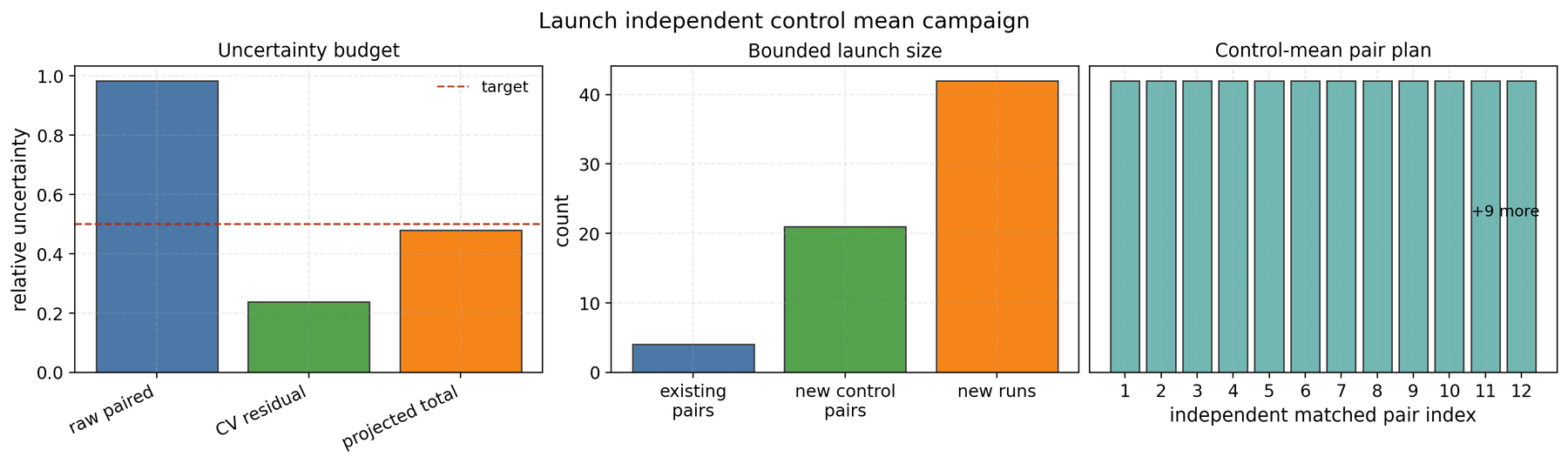
QA/ESS ZBS(1,0) rel7.5 independent control-mean campaign plan. The uncertainty budget shows the raw paired response, the screened control-variate residual, and the projected combined uncertainty after adding the independent control-mean estimate. The launch size is bounded at 21 matched plus/minus pairs, or 42 new nonlinear runs.

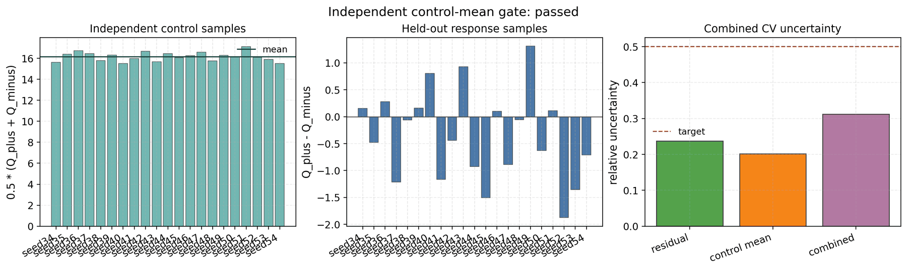
QA/ESS ZBS(1,0) rel7.5 independent control-mean gate. The completed office campaign uses 21 matched plus/minus seed pairs and the late post-transient window t=[600,1100]. Both state ensembles pass their spread and per-seed convergence gates, and the combined response uncertainty is 0.311 < 0.5. This closes the independent control-mean blocker for this specific variance-reduced nonlinear-gradient evidence lane.

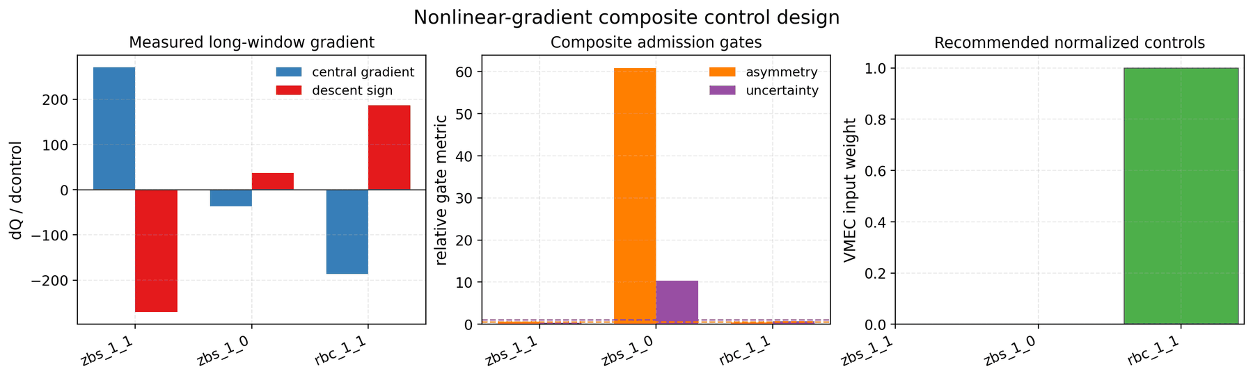
Nonlinear-gradient composite-control admission gate. The left panel shows the measured long-window central gradients and the corresponding descent signs, the middle panel shows locality and uncertainty admission gates, and the right panel shows the VMEC input weights that would be passed to the profile-direction writer. The current artifact intentionally fails closed: only RBC(1,1) is local, resolved, and sign-robust enough to enter the composite direction. ZBS(1,1) is still nonlocal, and ZBS(1,0) is unresolved and nonlocal, so the next production campaign needs another local/resolved control or a checked single-control bracket before long nonlinear GPU runs.

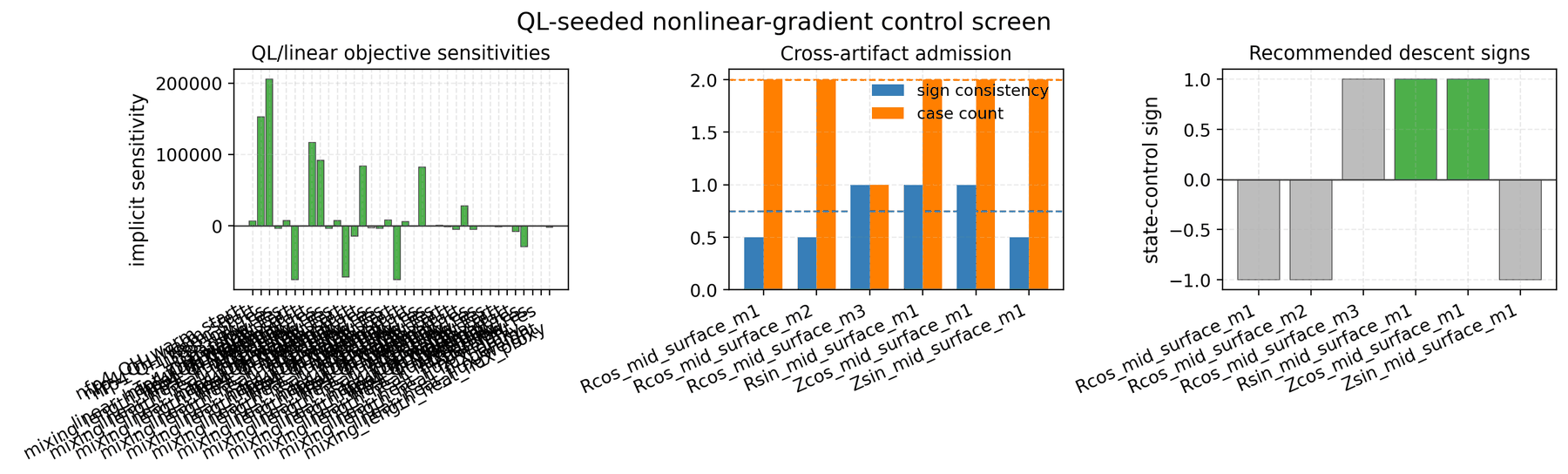
Quasilinear-seeded nonlinear-gradient control screen. This upstream gate uses full-chain vmex state sensitivities to decide which controls should even be considered for nonlinear long-window finite differences. The current QH/Li383 screen is now an upstream seed-admission gate only, not a nonlinear launch gate. The tracked Rcos and Zsin controls remain fail-closed because their primary quasilinear-proxy signs are not robust across the two equilibria, while Rsin_mid_surface_m1 and Zcos_mid_surface_m1 are admitted with two-case sign consistency. This is still an upstream control-admission result; a separate state-to-input mapping gate must pass before checked nonlinear bracket runs, and neither artifact is a converged nonlinear transport-gradient or optimized-equilibrium claim.

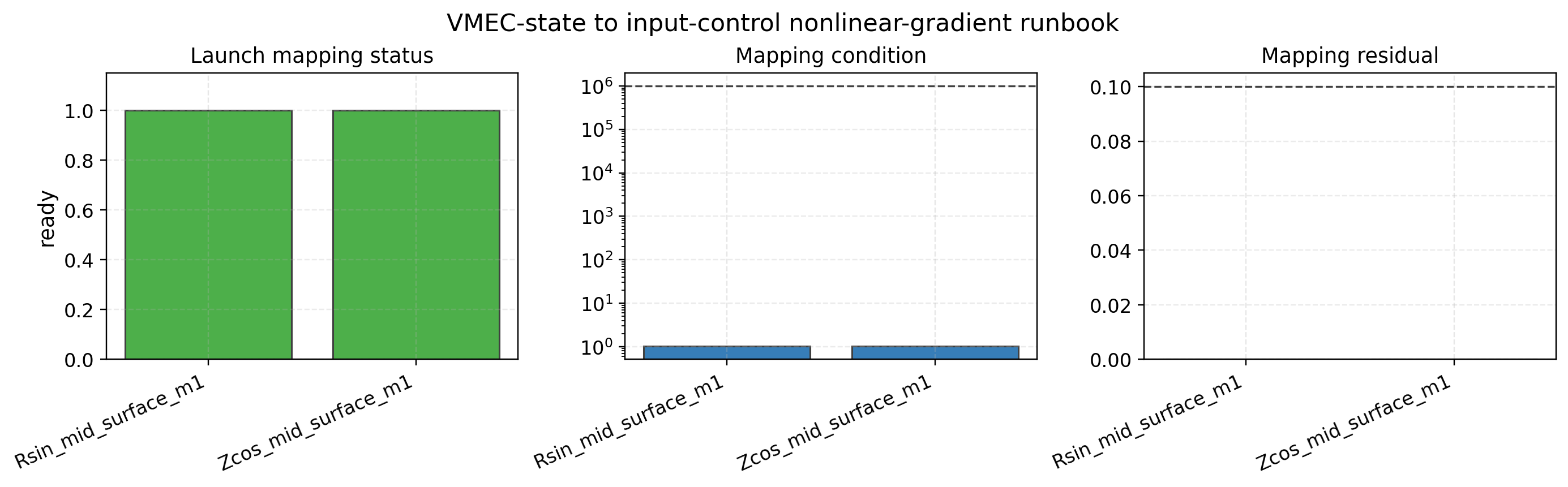
VMEC-state to input-control nonlinear-gradient runbook. This guardrail is the step between the QL seed screen and any nonlinear-gradient launch. It now passes only after the LASYM=true asymmetric state-to-input response artifact is attached. The accepted controls are least-squares combinations of four explicit RBS/ZBC VMEC input coefficients with a measured response condition number about 1.02 and residuals near machine precision. This closes the launch-mapping guardrail for checked short-bracket nonlinear runs; converged long-window nonlinear-gradient evidence remains a separate gate.

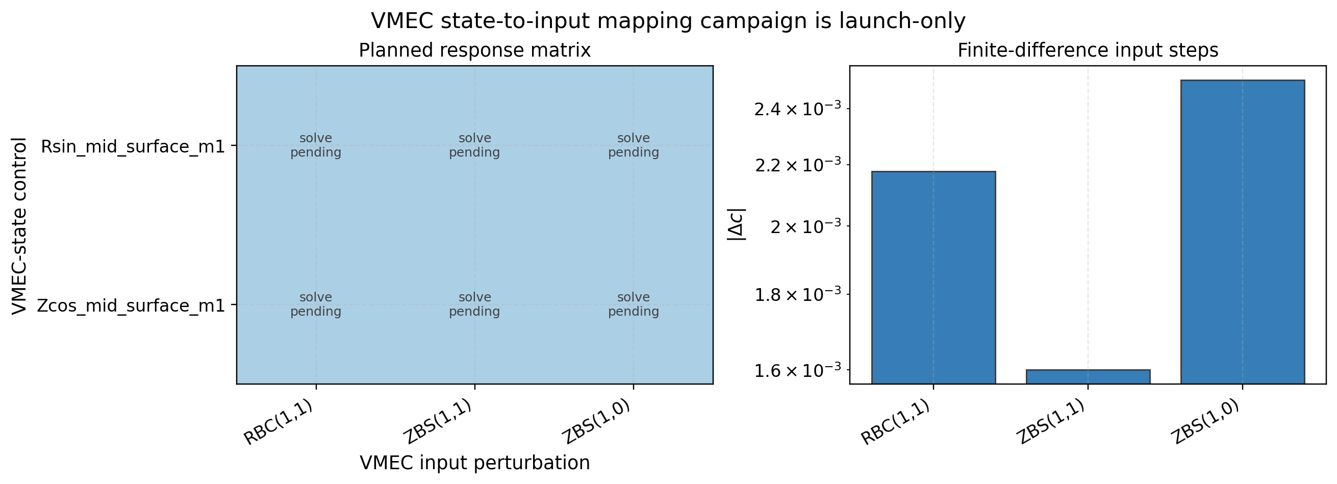
VMEC state-to-input mapping campaign launch plan. This is the concrete next-step artifact after the fail-closed runbook: it writes candidate RBC(1,1), ZBS(1,1), and ZBS(1,0) perturbation decks from a bundled QA VMEC input and records the response matrix that must be measured after re-equilibration. The blank matrix cells are labeled solve pending because this figure is not mapping evidence; it becomes useful for nonlinear launches only after the VMEC response extraction produces a conditioned, residual-bounded state-to-input mapping artifact.

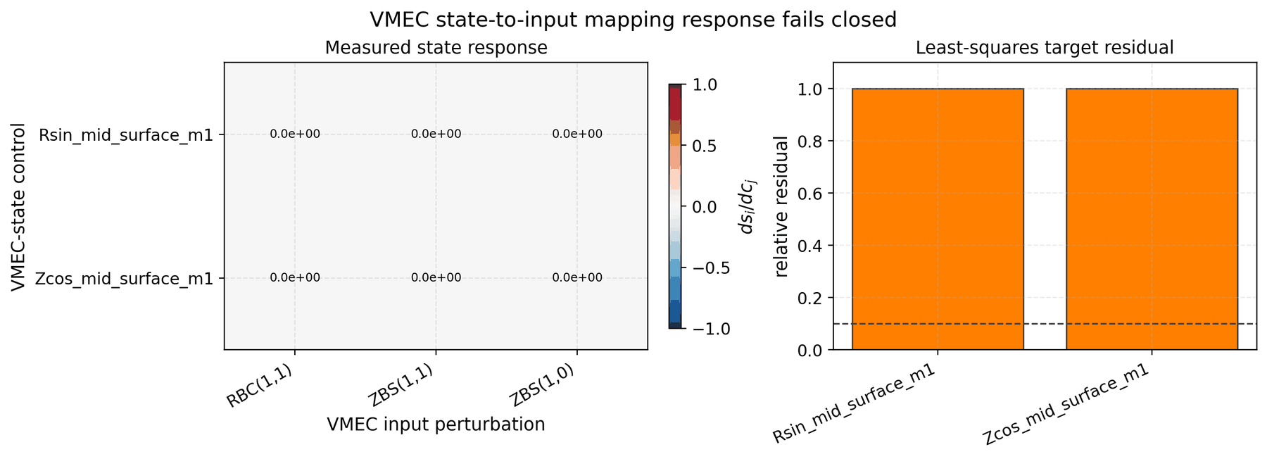
VMEC state-to-input measured response matrix. The nine baseline/plus/minus vmex solves terminated normally with the stricter explicit iteration budget, but the measured response of the admitted Rsin/Zcos controls to the stellarator-symmetric RBC/ZBS directions is identically zero. The least-squares target residual remains 1 for both controls, so this is a negative mapping result rather than launch evidence. The next viable branch must either use explicit LASYM=true RBS/ZBC controls or re-screen controls that live in the stellarator-symmetric subspace.

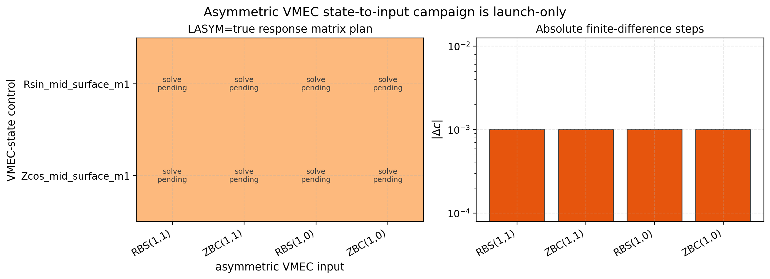
Asymmetric VMEC state-to-input mapping campaign launch plan. This follow-up uses the same QA input deck but writes LASYM=true baseline/plus/minus decks for four zero-baseline RBS/ZBC coefficients with absolute 1e-3 finite-difference steps. The figure remains a launch-plan artifact until the generated equilibria are solved and the response matrix is measured.

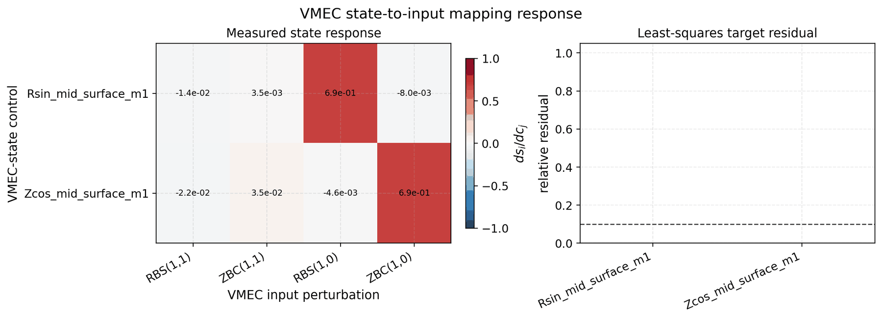
Asymmetric VMEC state-to-input measured response matrix. The twelve LASYM=true vmex solves terminated normally, and the measured response from RBS/ZBC input coefficients to the admitted Rsin/Zcos state controls has rank 2 with condition number about 1.02. The least-squares residuals are near machine precision, so this artifact can be attached to the runbook to produce explicit short-bracket launch directions.

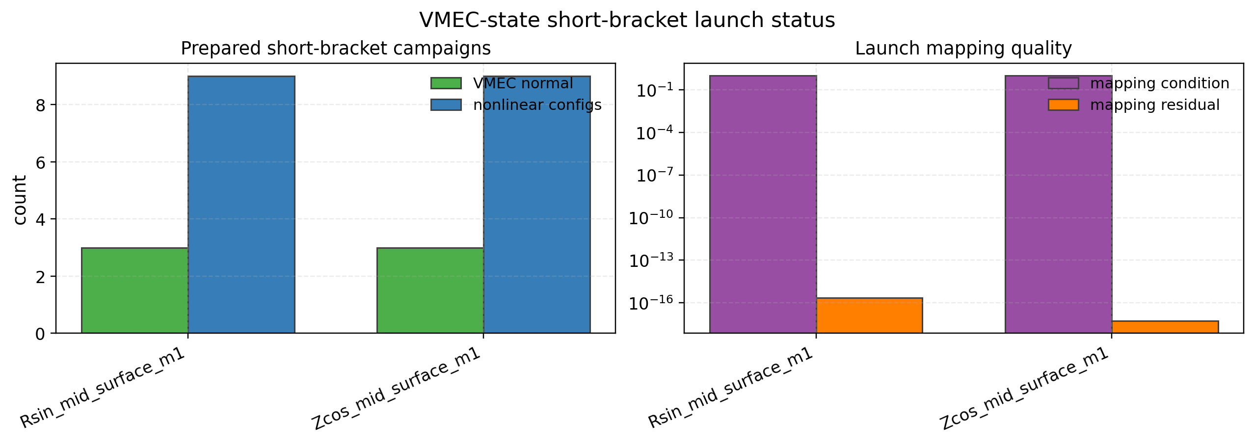
VMEC-state short-bracket launch status. The passing runbook is converted into two explicit LASYM=true VMEC input directions, one for each admitted state control. All six baseline/plus/minus VMEC decks terminate normally, and the bounded t=150 nonlinear campaign manifests are prepared. This panel documents readiness for the next nonlinear audit only; it is not a nonlinear-gradient or turbulent-flux promotion.

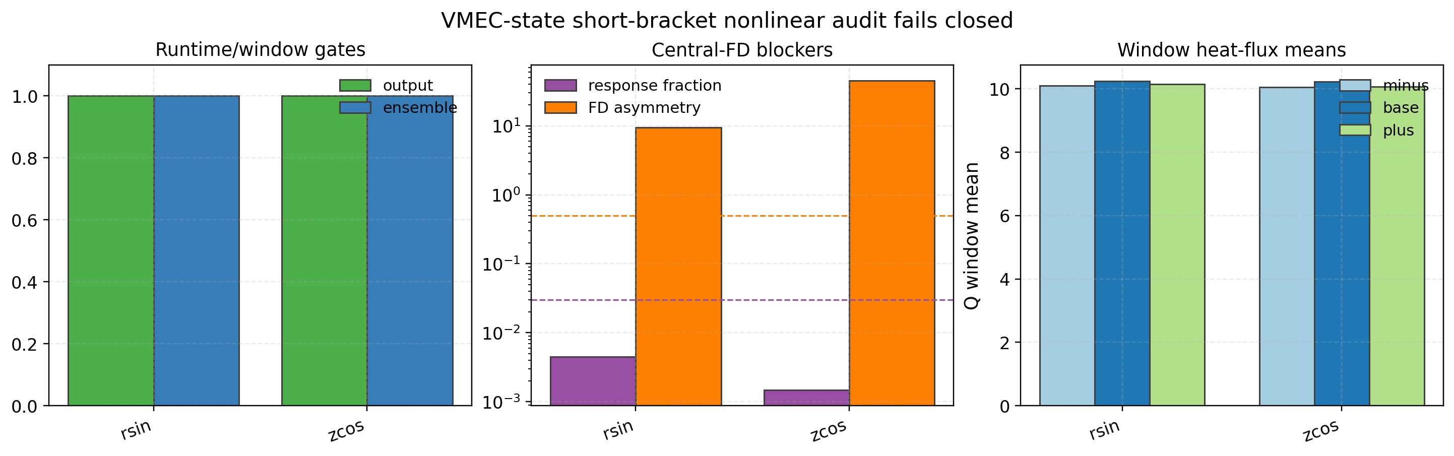
VMEC-state short-bracket nonlinear audit status. The prepared campaigns run on the office GPUs and produce all 18 nonlinear outputs. Runtime-output and replicated-window gates pass, with heat-flux means near 10 over t=[75,150]. The central finite-difference gates fail closed because the 1e-3 state-control step produces response fractions well below the 0.03 promotion threshold and large plus/minus asymmetry. The next evidence step is therefore a bracket-amplitude sweep, not a transport-gradient promotion.

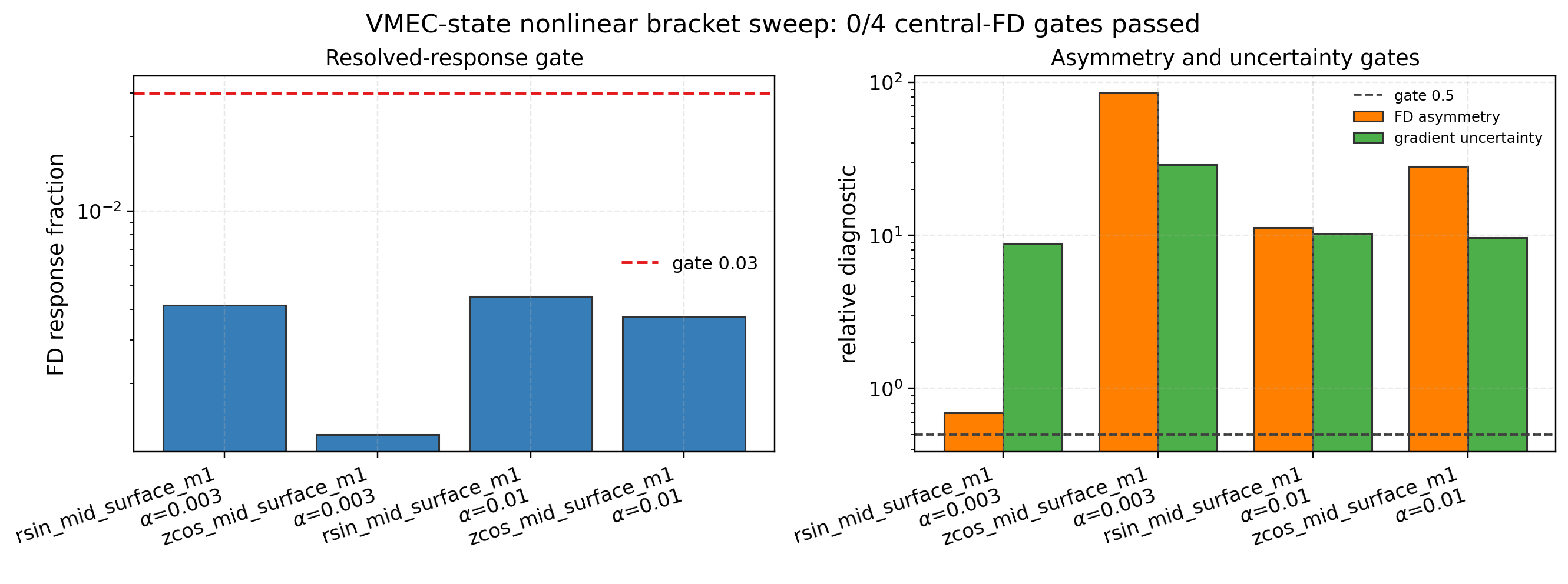
VMEC-state bracket-amplitude sweep status. The follow-up campaign runs both mapped controls at alpha_delta=3e-3 and 1e-2. All 36 nonlinear outputs complete on the office GPUs and the window/ensemble gates remain stable, but none of the four central finite-difference gates pass. The response fractions remain below 0.005 while the resolved-response gate is 0.03. This is negative evidence against simply increasing the single-control bracket; the next path is variance reduction or a better-conditioned multi-control observable.

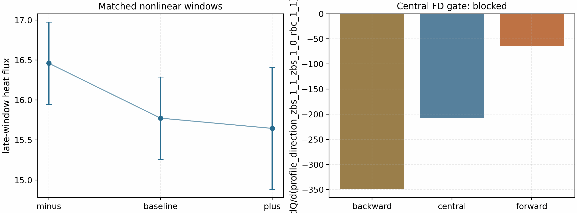
QA/ESS composite profile-direction nonlinear-gradient audit. The nine matched t=900 nonlinear runs all pass runtime-output gates; baseline and minus ensembles pass their replicated-window gates, but the plus ensemble has too much replicate spread. The finite-difference response is resolved but nonlocal and too uncertain, so the result is retained as fail-closed evidence for the next campaign design rather than a promoted gradient.

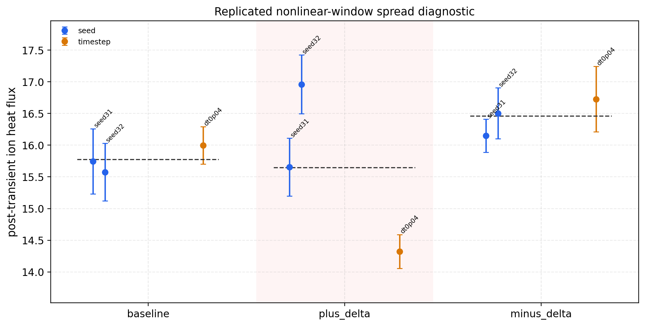
QA/ESS composite profile-direction replicate-spread diagnostic. The baseline and minus states remain within the seed/timestep spread gate, while the plus state fails because the high window is the seed32 run and the low window is the dt0p04 timestep run. This mixed seed/timestep failure is exactly the case where the correct action is not to add blind replicas at the same bracket: the next campaign must first separate timestep sensitivity from seed sensitivity or shrink the finite-difference bracket.

The targeted follow-up launch artifact for that decision is docs/_static/qa_ess_descent_profile_rel2_plus_delta_replicate_followup_plan.json. It kept the nonlinear-gradient claim fail-closed and wrote only three plus_delta cross variants: seed22_dt0p05 tested whether the low window followed the seed at the nominal timestep, seed32_dt0p04 tested whether the high window persisted at the refined timestep, and seed33_dt0p05 added one fresh nominal-timestep seed. Those runs have now completed on the office GPUs. All six plus_delta outputs pass the runtime-output gate, but the extended plus ensemble still fails the spread gate: mean_rel_spread = 0.166 > 0.15. The recomputed central finite-difference artifact therefore remains blocked by the plus ensemble, by fd_asymmetry_rel = 2.84 > 0.5, and by gradient_uncertainty_rel = 1.22 > 0.5. This closes the blind-replica question: more of the same plus-state runs are not the right next step. The next scientifically useful campaign should shrink the finite-difference bracket or use an overdetermined/profile-gradient design with matched seed/timestep labels across all parameter states.

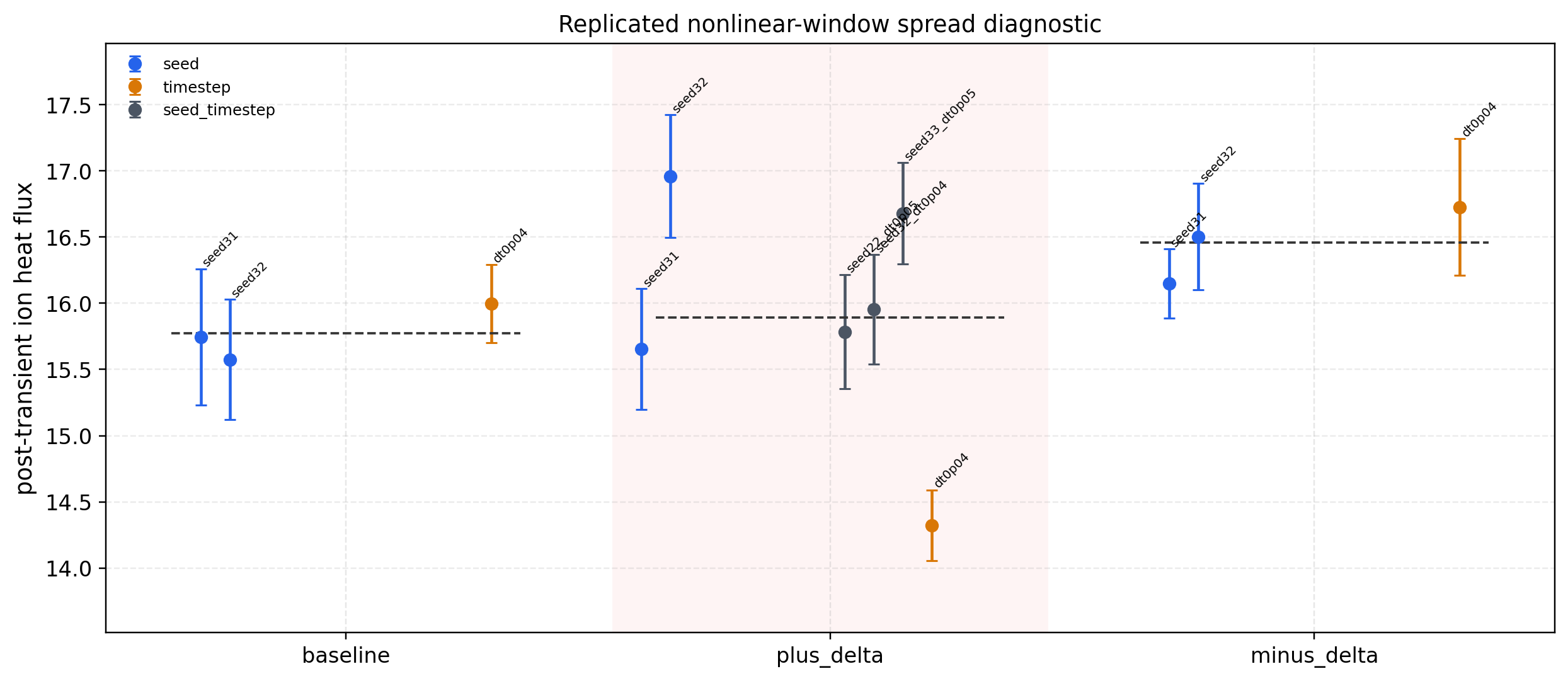
Targeted plus_delta follow-up for the QA/ESS composite profile-direction nonlinear-gradient audit. The baseline and minus states remain within the replicate-spread gate, but the expanded plus-state ensemble still exceeds the spread threshold after crossing seed and timestep variants. The shaded plus-state panel is the reason the nonlinear turbulence-gradient claim stays fail-closed.

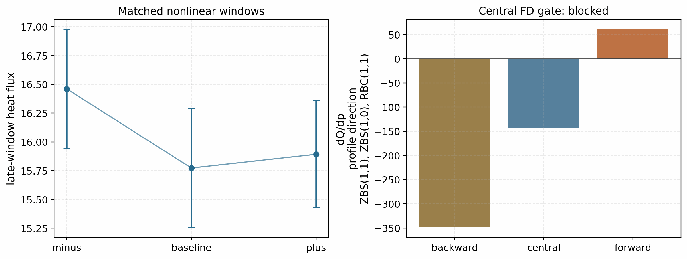
Central finite-difference audit after the targeted plus-state follow-up. The mean response is resolved, but the forward/backward finite differences are inconsistent and the propagated uncertainty is too large. This is recorded as a bounded negative result, not as nonlinear turbulence-gradient evidence.

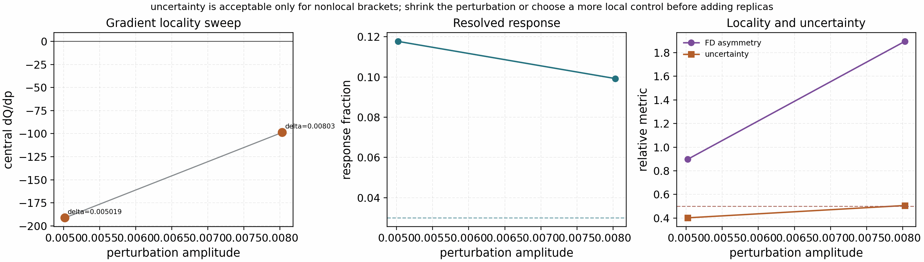
QA/ESS RBC(1,1) same-control perturbation-amplitude sweep. The two completed long-window central-FD artifacts show that increasing the perturbation amplitude does not improve locality: the response remains resolved, but the forward/backward asymmetry grows. This keeps the single-control RBC(1,1) path fail-closed and supports the move to a smaller locality sweep or an overdetermined profile-gradient campaign.

For boundary-coefficient gradients, the central finite-difference gradient JSON is supplied to tools/release/check_nonlinear_optimization_gates.py gradient-evidence together with the matched baseline, plus_delta, and minus_delta replicated ensemble artifacts. That gate checks the response fraction, forward/backward asymmetry, subtraction condition number, and propagated gradient_uncertainty_rel, and only that paired long-window workflow can promote a nonlinear turbulence-gradient claim.