Quasilinear Transport
GKX can compute quasilinear transport diagnostics from a linear eigenstate or late-time linear state. The implementation deliberately separates the exact linear diagnostic from any saturation model:
linear weights are amplitude-normalized heat and particle fluxes computed with the same diagnostic kernels used by runtime simulations;
saturation rules are named, serialized model assumptions that convert a linear mode into a trend-level saturated estimate;
calibrated absolute flux claims require nonlinear training and holdout validation and should not be inferred from the uncalibrated rules alone.
Current validated scope
The current implementation supports electrostatic channels only:
[quasilinear]
enabled = true
mode = "weights"
saturation_rule = "none"
amplitude_normalization = "phi_rms"
kperp_average = "phi_weighted"
channels = ["es"]
The diagnostic writes:
*.quasilinear.summary.jsonwith growth rate, frequency, normalization,kperp_eff2, species weights, and saturation metadata;*.quasilinear_species.csvwith species-resolved heat and particle flux weights and, when requested, saturated estimates.*.quasilinear_spectrum.csvfor serialscan-runtime-linearruns with quasilinear diagnostics enabled.
For linked-boundary or imported-geometry scans, *.quasilinear_spectrum.csv
stores two perpendicular-mode coordinates: ky is the requested scan
coordinate used for ordering and plotting, while mode_ky is the selected
signed grid-mode coordinate used internally by the linear solve. This prevents
negative-branch aliases from corrupting publication spectra while preserving
the exact selected mode metadata.
Literature anchors and claim policy
The GKX quasilinear layer follows the same separation used in modern reduced gyrokinetic transport workflows:
the linear gyrokinetic eigenproblem determines growth rates, frequencies, eigenfunctions, cross-phases, and species-resolved flux weights;
a separate saturation rule converts those linear quantities into fluctuation amplitudes;
nonlinear simulations or experimental transport databases are required before claiming calibrated absolute fluxes.
This separation is central to early nonlinear tests of quasilinear transport models [Waltz09], to the QuaLiKiz derivation [Stephens21], to profile- evolution use cases [Citrin17], and to broader quasilinear-model validation reviews [Staebler24]. Parker et al. [Parker23] show why saturation rules must be treated as model assumptions rather than consequences of the linear solve alone. SAT3 [Dudding22] and SAT3-NN [Sar26] are useful longer term targets because they use spectrum-aware, database-calibrated saturation information instead of a single uncalibrated mixing-length constant.
For stellarator optimization, GKX currently treats quasilinear fluxes as
research diagnostics and optimization proxies, following the microstability
optimization motivation in [Jorge24]. The present release does not claim a
validated absolute nonlinear flux predictor. The current 12-case
train/holdout calibration portfolio validates the input plumbing and rejects
the one-constant saturation-rule family, with CTH-like and shaped-pressure external VMEC
admitted only through explicit high-grid policies and QP and Solovev admitted
through replicated seed/timestep ensembles. The QI candidate remains negative evidence:
it is finite at t=250 but its n48/n64 late-window heat-flux means differ
by about 0.38, above the 0.15 grid/window gate. The simple-rule and
candidate-model sweeps have been regenerated on that expanded ledger. The
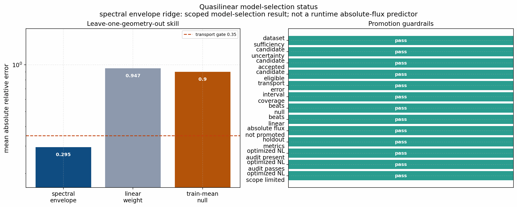
richer spectral_envelope_ridge candidate is the least-bad reduced model,
but it misses the strict transport and rank-screening gates; it is not exposed
as a runtime saturation law or universal transport model.
Scoped core and universal-stress verdict
This lane is closed as a scoped core-portfolio quasilinear diagnostic and keeps the full-ledger universal absolute-flux claim deferred. The independent-holdout-count blocker is closed: the frozen ledger has two training references and ten admitted holdouts. The declared stress outliers are the Solovev repaired external-VMEC case and the shaped-pressure external-VMEC case. They remain in the residual-anatomy artifact as negative stress-case evidence, but they are outside the current core claim.
The tested one-constant family has the form
where gamma and kperp_eff2 come from the linear solve and
Qhat is the amplitude-normalized heat-flux weight. The scalar
C_sat is fitted only on the training cases by through-origin least squares,
The promotion gate is fail-closed:
with nonlinear windows admitted only after finite late-time traces,
running-mean drift checks, uncertainty/replicate checks where applicable, and
grid/time-window convergence gates. The current positive-growth mixing-length
model gives held-out mean relative error about 6.49; the simple
linear-weight fit gives 4.42; the absolute-growth diagnostic gives
6.85; and the training-mean null gives 1.80. The best reduced
candidate, spectral_envelope_ridge, reaches leave-one-geometry-out mean
relative error about 0.697 with interval coverage 11/12; its held-out
screening metrics are Spearman = 0.624 and pairwise order accuracy
0.689. On the declared 10-case core portfolio, the same candidate passes
the scoped transport and coverage gate: mean relative error is about 0.280,
held-out mean relative error is about 0.275, maximum relative error is
about 0.575, and interval coverage is 10/10. The core rank-screening
metric remains borderline (full-core Spearman about 0.745, just below the
0.75 gate). GKX therefore ships this as a scoped core diagnostic
and optimization-screening tool, not as a universal nonlinear heat-flux
predictor or runtime saturation law.
Executable usage
gkx run-runtime-linear \
  --config examples/linear/axisymmetric/runtime_cyclone_quasilinear.toml \
  --out tools_out/cyclone_quasilinear
or enable the diagnostic for another linear runtime TOML:
gkx run-runtime-linear \
  --config examples/linear/axisymmetric/cyclone.toml \
  --quasilinear \
  --ql-mode saturated \
  --ql-saturation-rule mixing_length \
  --ql-normalization phi_rms \
  --ql-csat 1.0 \
  --out tools_out/cyclone_quasilinear
For a ky spectrum, use the independent-scan path. --workers can
parallelize the per-ky linear solves and quasilinear state extraction while
preserving the serial ordering of the output spectrum:
gkx scan-runtime-linear \
  --config examples/linear/axisymmetric/runtime_cyclone_quasilinear.toml \
  --ky-values 0.1,0.2,0.3,0.4 \
  --quasilinear \
  --workers 2 \
  --out tools_out/cyclone_quasilinear_scan
Then render the spectrum:
python tools/artifacts/plot_quasilinear_diagnostics.py spectrum \
  --spectrum tools_out/cyclone_quasilinear_scan.quasilinear_spectrum.csv \
  --out docs/_static/quasilinear_cyclone_spectrum.png
The shipped worker-identity gate for this path is generated with:
JAX_ENABLE_X64=1 python tools/artifacts/generate_parallel_identity_gate.py quasilinear-runtime \
  --workers 2 \
  --ky 0.1 0.2 \
  --out-prefix docs/_static/quasilinear_runtime_parallel_gate
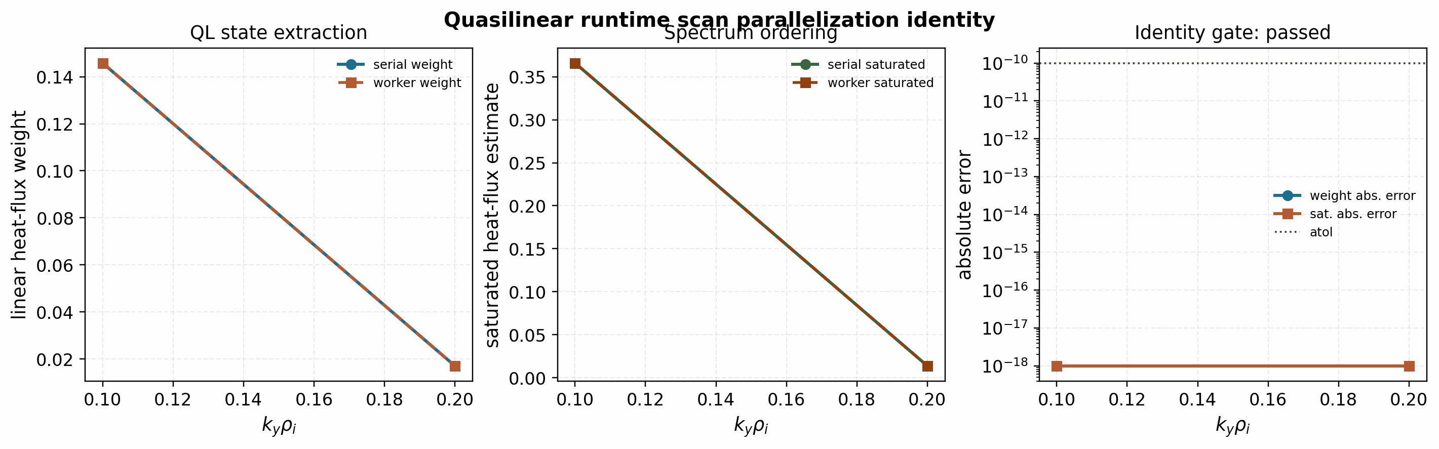
Serial and worker-parallel scan-runtime-linear quasilinear spectra from
the same runtime configuration. The gate checks ordered state-extraction
identity for the linear heat-flux weight and the saturated heat-flux
estimate; any timing metadata is reported for engineering tracking only,
not as a production speedup claim.
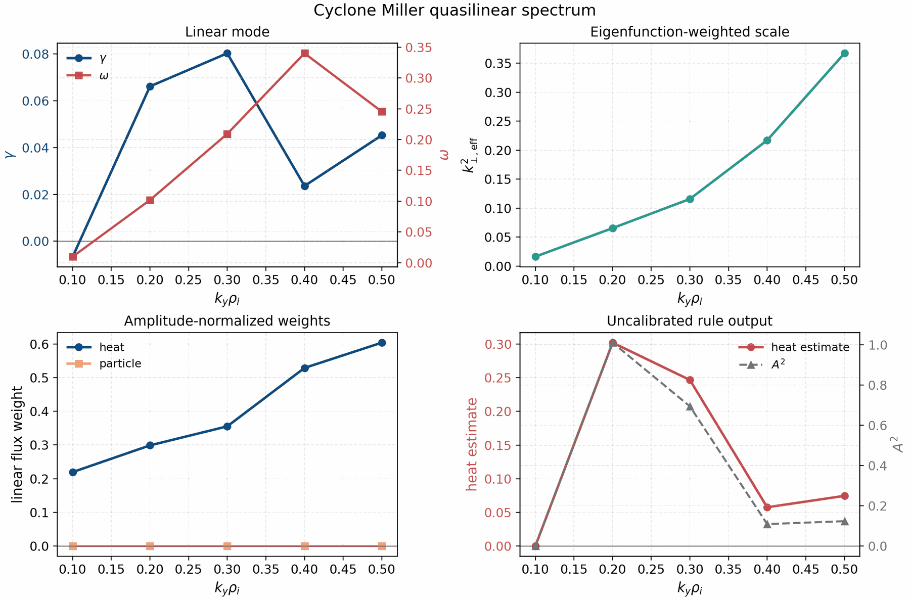
The shaped-tokamak Miller companion uses the same pattern, with the positive
ky range resolved by the nonlinear run’s Ny=64 grid:
gkx scan-runtime-linear \
  --config examples/linear/axisymmetric/runtime_cyclone_miller_quasilinear.toml \
  --ky-values 0.1,0.2,0.3,0.4,0.5 \
  --quasilinear \
  --out docs/_static/quasilinear_cyclone_miller_spectrum_scan
Model details
Linear eigenproblem
For a fixed flux-tube geometry and perpendicular mode, the linear runtime solves the matrix-free system
where G is the Hermite-Laguerre gyrocenter moment state, v_j is a right
eigenvector, and
The sign convention above matches the runtime output: gamma is the growth
rate and omega is the physical mode frequency reported by the executable.
The operator is assembled by
gkx.terms.assembly and the individual term modules under
gkx.terms.
Field solve and linear weights
Given a linear state G, GKX first reconstructs fields with
compute_fields_cached. In the currently validated electrostatic path the
quasilinear diagnostic uses phi and sets A_parallel = B_parallel = 0.
Electromagnetic quasilinear channels remain disabled until the field-channel
normalization and nonlinear-calibration gates are complete.
The species heat and particle weights are computed with the same diagnostic
kernels used for nonlinear runtime outputs. For the electrostatic heat-flux
channel, the code contracts the radial E x B velocity factor with the
Hermite-Laguerre pressure moment:
Here W_k includes the positive-ky Hermitian factor, the dealias mask, the
flux-surface Jacobian/grad rho weight, species density/temperature factors,
and the selected diagnostic flux scale. The particle-flux channel uses the
density moment
but it is zero for the one-ion adiabatic-electron cases because there is no
kinetic electron species carrying particle transport. The implemented formulas
live in gkx.diagnostics.heat_flux_species(),
gkx.diagnostics.particle_flux_species(), and
_heat_flux_channel_contrib_species in
gkx.diagnostics.
Amplitude normalization and effective scale
The implemented effective perpendicular scale is
where the average uses the runtime spectral and flux-tube volume weights. Heat and particle flux weights are divided by the selected amplitude normalization, making them invariant under eigenfunction phase rotations and amplitude rescalings.
The normalized linear weights are therefore
The default normalization is
with the same Hermitian and flux-tube weights used by
gkx.diagnostics.quasilinear_transport.spectral_phi_weights().
Supported amplitude normalizations are:
phi_rms: weighted|\phi|^2average;phi_midplane: maximum midplane|\phi|^2;field_energy: electrostatic field-energy normalization.
Supported saturation rules are:
none: write linear weights only;mixing_length:A^2 = C_sat max(gamma - gamma_floor, 0) / kperp_eff2;lapillonne_2011: currently the same audited scaling contract asmixing_lengthuntil the broader model-specific validation suite is added.linear_weight:A^2 = C_sat. This is a diagnostic intensity rule used to test whether the linear flux-weight spectrum alone transfers across geometries.absolute_growth_mixing_length:A^2 = C_sat |gamma| / kperp_eff2. This gives stable short-window branches nonzero diagnostic intensity and is included only for saturation-model stress tests, not as a validated physical rule.
The current mixing-length output is
This is intentionally the simplest possible baseline. It is useful for software validation and sensitivity studies, but Parker-style saturation-rule comparisons [Parker23], SAT3/SAT3-NN-style spectrum-aware rules [Dudding22] [Sar26], and nonlinear holdout tests are required before it can be used as a predictive absolute-flux model.
The reduced objective helper
gkx.diagnostics.quasilinear_transport.quasilinear_feature_objective supports the same
diagnostic rules for differentiability tests from feature vectors
[gamma, kperp_eff2, flux_weight]. The fast suite checks the resulting
Jacobians against central finite differences before these objectives are used
in optimization examples.
Implementation map
Layer |
Source |
Responsibility |
|---|---|---|
Quasilinear weights |
phase/amplitude-invariant |
|
Diagnostic kernels |
|
heat, particle, field-energy, volume-factor, and resolved flux contractions shared by linear and nonlinear paths |
Runtime plumbing |
|
single-run and scan execution, TOML/executable overrides, JSON/CSV artifact writing |
Input schema |
|
|
Calibration reports |
train/holdout/audit schemas, spectrum integration, nonlinear-window ingestion, scale fitting, and report scoring |
|
Plotting tools |
|
publication-facing spectrum and calibration figures |
Differentiability gates |
finite-difference checks, covariance diagnostics, dense operator fixtures, and implicit isolated-eigenpair sensitivities |
Algorithmic workflow
For one linear mode:
build grid, geometry, species, and linear cache
solve the linear eigenproblem or fit the late-time linear state
reconstruct phi from the eigenvector/state
compute kperp_eff2 from |phi|^2 weights
compute heat and particle flux contractions using runtime diagnostic kernels
divide by the requested amplitude normalization
optionally apply a named saturation rule
write summary JSON and species CSV artifacts
For a serial ky scan:
for requested ky in ky_values:
    select the closest grid mode
    run the single-mode linear solve
    compute quasilinear payload
    store requested ky and selected signed mode_ky
write *.scan.csv and *.quasilinear_spectrum.csv
For nonlinear calibration:
integrate or load nonlinear diagnostic CSV over a declared time window
compute late-window convergence metadata after transient removal
require finite mean, running-mean drift, block-bootstrap SEM, and provenance
integrate/sum the linear quasilinear spectrum
create train, holdout, or audit calibration points
optionally fit one multiplicative scale on train points only
score holdout points against explicit mean-relative-error and window gates
Numerics and differentiability
GKX production linear solves remain matrix-free. Dense matrices are
only materialized in tiny validation fixtures through
gkx.objectives.autodiff_validation.explicit_complex_operator_matrix().
Eigenvalue sensitivities use JAX derivatives of the matrix entries and the standard isolated-branch relation
where v and w are right and left eigenvectors. Eigenfunction-dependent
observables use the implicit perturbation system
The gauge condition w^\dagger \partial_i v = 0 makes the derivative unique
for phase-invariant observables. This path is now tested on a tiny
GKX linear-RHS fixture and compared against nearest-branch central
finite differences. Direct JAX differentiation through non-Hermitian
eigenvectors is
still explicitly guarded because JAX does not provide that JVP; the implicit
path is the supported validation route.
Validation gates
The fast test suite currently checks:
TOML and executable plumbing for
[quasilinear];phase and amplitude invariance of the linear weights;
explicit rejection of unvalidated electromagnetic channels;
artifact serialization for summary and species tables;
a small Krylov runtime smoke test.
autodiff-vs-finite-difference and tangent checks for the reduced mixing-length objective
[gamma, kperp_eff2, flux_weight].branch-isolated eigenvalue AD-vs-finite-difference checks, which are the lightweight gate used before differentiating full linear growth/frequency outputs.
a tiny dense GKX linear-RHS fixture that materializes the otherwise matrix-free operator, disables the production custom-VJP field solve for forward-mode validation, and checks an isolated eigenvalue derivative against central finite differences.
an explicit guard showing that direct JAX differentiation through non-Hermitian eigenvectors is unsupported;
an implicit left/right eigenpair sensitivity gate for phase-invariant eigenfunction observables, including a tiny GKX linear-RHS quasilinear-style objective checked against finite differences.
a fast promotion guardrail that scans the calibration/model-selection JSON reports, conservative documentation wording, and the manuscript-readiness quasilinear lane. A closed manuscript lane must remain explicitly scoped as a diagnostic/model-selection result and must list the guardrail artifact; it is not a calibrated absolute-flux claim.
Implicit sensitivity example
The user-facing example
examples/theory_and_demos/quasilinear_implicit_sensitivity.py applies the
implicit gate to a tiny Cyclone linear-RHS fixture. The differentiated
observable is
where Q_i^(ML) is the uncalibrated mixing-length heat-flux proxy computed
from the linear heat-flux weight. The parameter vector is
[R/L_n, R/L_Ti]. The goal is not to claim nonlinear-flux prediction from
this tiny fixture; the goal is to verify that a phase-invariant quasilinear
observable can be differentiated through an isolated non-Hermitian eigenbranch
without relying on unsupported JAX eigenvector derivatives.
python examples/theory_and_demos/quasilinear_implicit_sensitivity.py \
  --outdir docs/_static
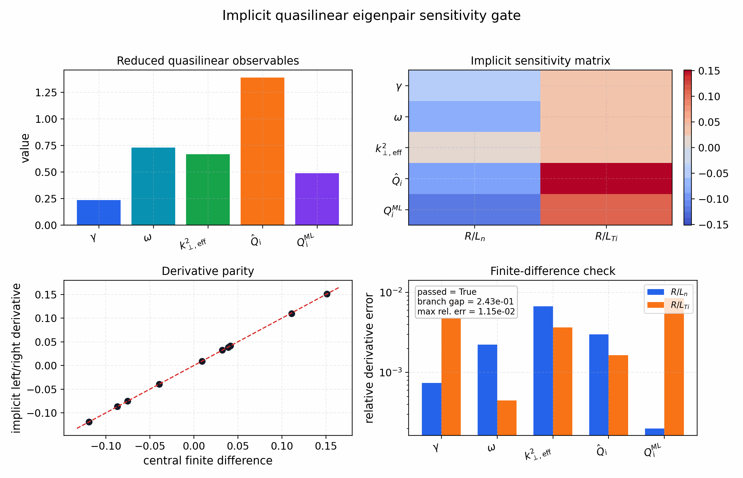
The lower panels compare the implicit left/right derivative against central
finite differences that follow the nearest isolated eigenvalue branch. The
tracked artifact passes with maximum relative derivative error around
1.2e-2 and branch gap around 2.4e-1. Those values are stored in
docs/_static/quasilinear_implicit_sensitivity.json so documentation figures
and tests use the same audit payload.
The manuscript-level validation plan adds nonlinear calibration and holdout studies across axisymmetric and stellarator cases before making absolute transport-prediction claims. The model and calibration policy follows the quasilinear derivation and saturation-rule validation philosophy in [Stephens21] and [Parker23].
Calibration reports
Calibration artifacts should use
gkx.diagnostics.quasilinear_calibration so training, holdout, and
audit points carry the same schema. A report is promoted
to calibrated_absolute_flux only when it contains at least one training
point, at least one holdout point, finite passed nonlinear late-window
convergence metadata for every holdout, and the holdout mean-relative-error
gate passes. The window metadata comes from
gkx.diagnostics.transport_windows or
tools/release/check_nonlinear_transport_gates.py convergence and records the transient
cutoff, late-window mean/std, running-mean drift, block/bootstrap SEM, sample
counts, and source-artifact provenance. Otherwise the claim is demoted to
calibration_dataset or training_or_audit_only. This keeps README, docs,
and manuscript figures from claiming absolute nonlinear transport prediction
from an uncalibrated
saturation rule.
Replicated nonlinear windows should additionally be checked with
gkx.diagnostics.transport_windows.nonlinear_window_ensemble_report before they
are used as seed, initial-condition, or timestep-robust transport evidence.
The ensemble gate consumes already-built nonlinear-window convergence reports,
requires each input window to be promotion-ready by default, and checks the
relative spread of late-window means plus the combined SEM across replicates.
This is the lightweight metadata gate that lets the validation ladder state
that several long nonlinear runs agree; it is not a substitute for actually
running those long nonlinear simulations. The command-line artifact wrapper is
tools/release/check_nonlinear_transport_gates.py ensemble; it reads multiple window JSON
reports and writes a JSON report plus an optional PNG summary for documentation
or manuscript audit trails.
For a matched intervention such as equilibrium flow shear, first build one
convergence report per trace and then run
tools/release/check_nonlinear_transport_gates.py matched-windows. This final
gate requires both windows to pass before evaluating relative reduction and its
quadrature-SEM separation; it therefore cannot promote a lower but still
drifting treatment mean.
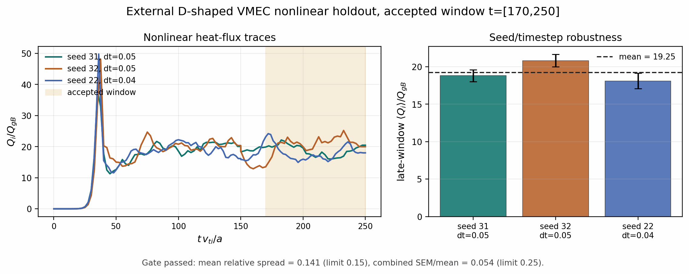
The first tracked external-VMEC replicate campaign applies that protocol to
the admitted D-shaped nonlinear holdout. Six office-GPU runs were launched from
the same n64 configuration family: t=150 startup runs and t=250
continuations for seeds 31 and 32 at dt=0.05, plus a timestep
variant with seed 22 at dt=0.04. The late transport window
t=[170,250] passes the readiness gate and the ensemble gate without
relaxing the spread or uncertainty thresholds: the accepted means are about
18.8, 20.8, and 18.1 in gyro-Bohm units, the mean-relative spread is
0.141 against the 0.15 gate, and the combined SEM/mean is 0.054
against the 0.25 gate. This strengthens the D-shaped holdout as nonlinear
model-development evidence; it still does not promote the current quasilinear
model to an absolute saturated-flux predictor.
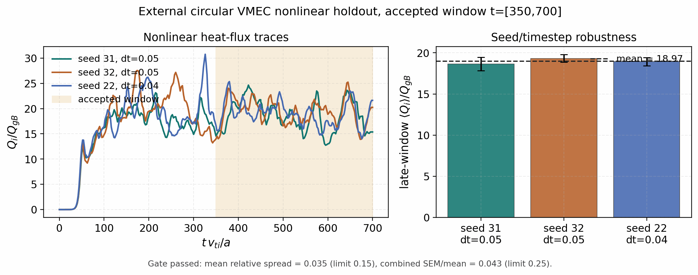
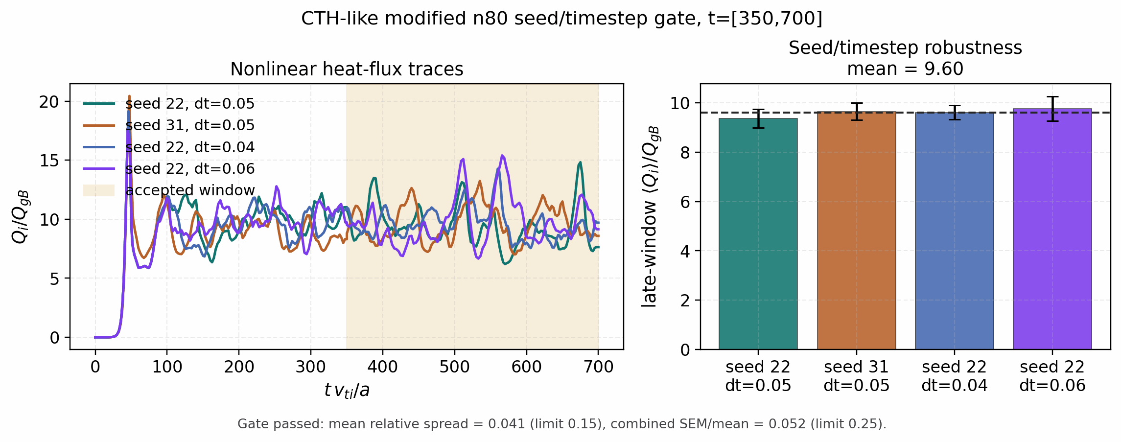
The next independent external-VMEC replicate campaign uses the admitted
circular tokamak holdout. The first t=450 pass was intentionally not
promoted even though the seed/timestep ensemble spread was small
(mean_rel_spread≈0.076): seed 31 failed terminal-window agreement
(0.199 against the 0.15 gate), showing that the late-time heat flux
was still drifting. Extending the same three replicas to t=700 and using
the later t=[350,700] window closes the readiness and ensemble gates
without relaxing thresholds. The accepted means are consistent across seed
and timestep variants, with ensemble mean 18.97, mean-relative spread
0.035, and combined SEM/mean 0.043. This is the circular holdout’s
replicated nonlinear-window artifact; the failed t=450 readiness result is
retained as convergence-history evidence rather than a promoted figure.
The report builder is intentionally strict. Every point in one report must use
the report’s named saturation_rule; predicted fluxes, observed nonlinear
window means, and optional window standard deviations must be finite; and
window standard deviations must be non-negative. Spectrum integration similarly
rejects missing columns, all-non-finite samples, invalid integration methods,
and non-positive delta_ky widths. These checks are part of the validation
surface: a quasilinear figure can be exploratory, but a calibration or
candidate-model artifact cannot silently mix rules or admit non-converged,
non-finite, or dimensionally ambiguous data.
Train and holdout points must also be tied to a passed nonlinear validation
gate before they can be used in calibration. The audit tool
tools/release/check_quasilinear_promotion_guardrails.py calibration-inputs enforces that rule by matching
each point’s nonlinear_artifact to tracked nonlinear gate metadata. It
passes for the current Cyclone, Cyclone Miller, HSX, W7-X, D-shaped
external-VMEC, ITERModel, up-down asymmetric, circular, high-grid-admitted
CTH-like, and high-grid-admitted shaped-pressure external-VMEC calibration
inputs in the 12-case portfolio. The CTH-like and shaped-pressure rows are
matched through explicit high-grid admission gates rather than through failed
coarse-grid pilots. The same audit would still fail if an exploratory or
non-converged pilot such as the older CTH-like feasibility trace were inserted
directly as a train/holdout point.
The companion audit tools/release/check_quasilinear_promotion_guardrails.py is the
metadata promotion guard: it requires finite nonlinear window means and
standard deviations, train/holdout artifact provenance, passed held-out gates
before calibrated_absolute_flux promotion, and explicit documentation scope
markers. It also audits the manuscript quasilinear model-development figure
index: each tracked figure must have a JSON sidecar, a scoped non-absolute
claim level, explicit failed-baseline or blocker metadata where relevant, and
README/docs wording that does not promote a runtime/TOML absolute-flux
predictor. The current tracked reports are therefore not a calibrated
absolute-flux claim.

Existing nonlinear window summaries can be converted into calibration points
with calibration_point_from_nonlinear_window_summary when the summary points
to either a diagnostics CSV or a GKX runtime NetCDF file. CSV inputs use
the t column and the selected heat-flux column, usually heat_flux.
NetCDF inputs use Grids/time and map heat_flux to
Diagnostics/HeatFlux_st; heat_flux_es, heat_flux_apar, and
heat_flux_bpar map to the corresponding Diagnostics/HeatFlux*_st
variables. Species are summed by default for NetCDF variables with shape
(time, species); pass --species-index to the report builder when an
ion-only or electron-only nonlinear target is needed. The helper uses the
summary’s tmin/tmax window when present, otherwise the full finite time
range, and records the mean and standard deviation of the selected heat-flux
observable.
python tools/artifacts/plot_quasilinear_calibration.py report \
  --points docs/_static/quasilinear_calibration_points.json \
  --out docs/_static/quasilinear_calibration_report.json \
  --saturation-rule mixing_length
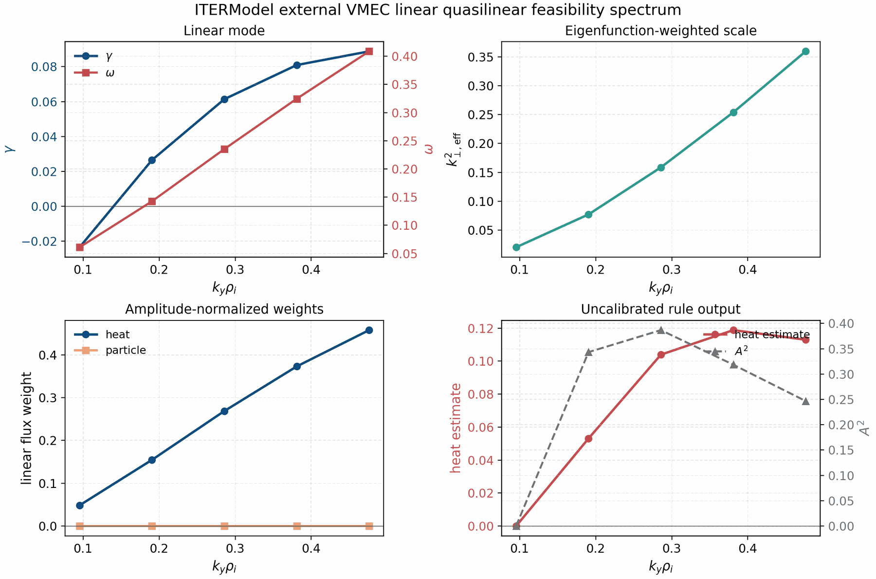
The first tracked audit point maps the Cyclone quasilinear spectrum above to
the long-window nonlinear Cyclone heat-flux diagnostic. It is intentionally an
audit point, not a calibrated transport claim:
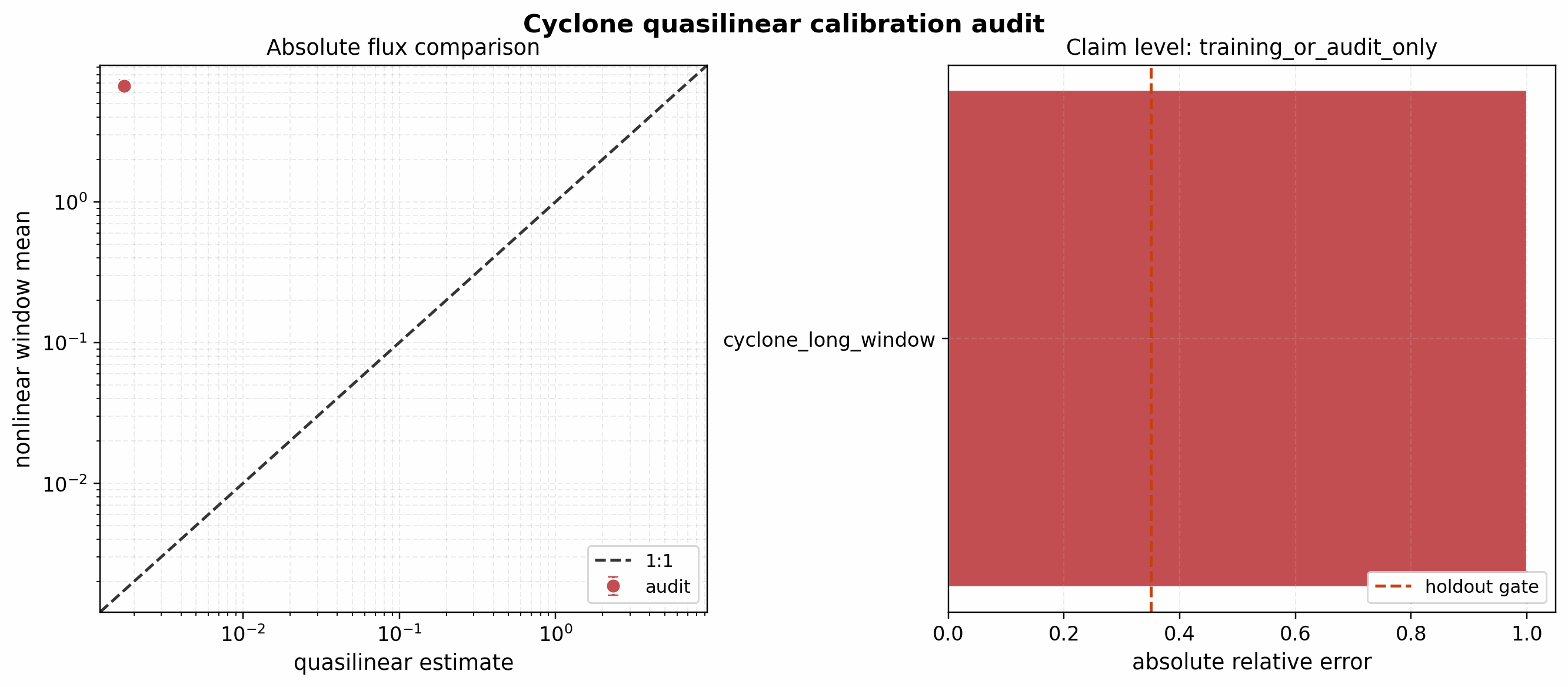
With C_sat = 1 the simple mixing-length rule underpredicts the absolute
nonlinear heat flux by orders of magnitude. This is the expected outcome for an
uncalibrated saturation rule and is precisely why the report remains at
training_or_audit_only. A paper-level absolute-flux claim requires a
documented training set, held-out nonlinear cases, and passed holdout gates.
The same report can also be generated directly from a quasilinear spectrum and a nonlinear gate summary:
python tools/artifacts/plot_quasilinear_calibration.py report \
  --spectrum docs/_static/quasilinear_cyclone_spectrum_scan.quasilinear_spectrum.csv \
  --nonlinear-summary docs/_static/nonlinear_cyclone_gate_summary.json \
  --split audit \
  --case cyclone_long_window \
  --geometry cyclone \
  --electron-model adiabatic \
  --saturation-rule mixing_length \
  --out docs/_static/quasilinear_cyclone_calibration_audit_report.json

python tools/artifacts/plot_quasilinear_calibration.py \
  --report docs/_static/quasilinear_cyclone_calibration_audit_report.json \
  --out docs/_static/quasilinear_cyclone_calibration_audit.png
Train/holdout transfer
The first geometry-transfer gate fits a single multiplicative heat-flux scale
on the Cyclone long-window nonlinear diagnostic and holds out the Cyclone
Miller nonlinear window. This is the minimal one-constant calibration expected
of a simple mixing-length saturation rule: if it fails, the missing ingredient
is not just a constant C_sat.
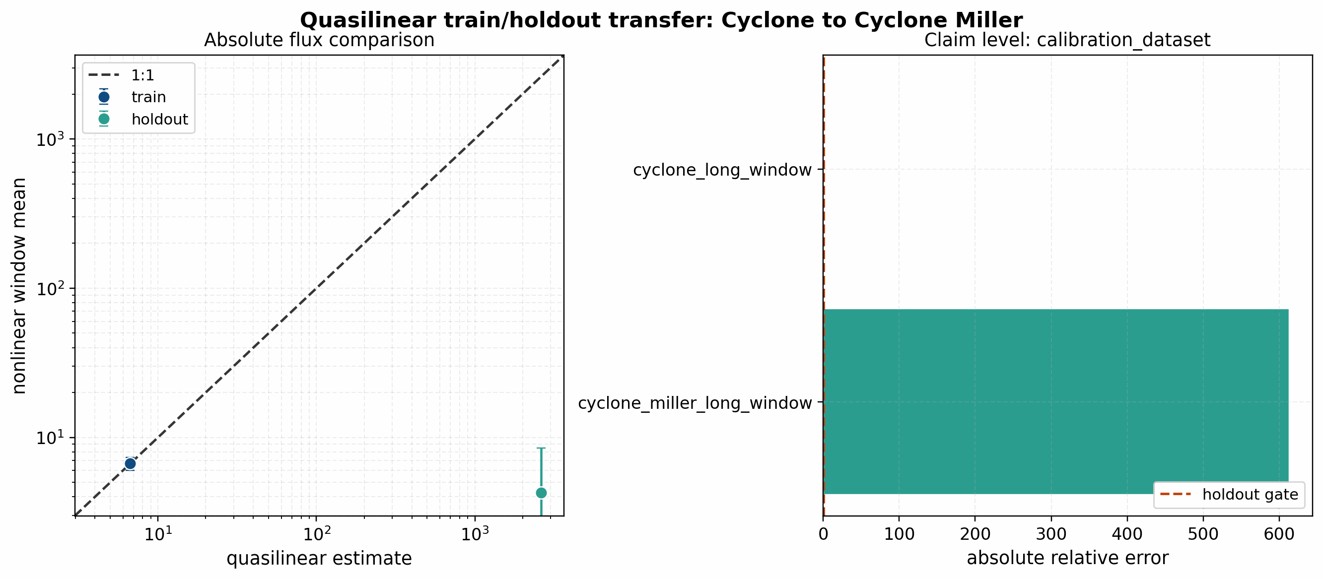
The tracked report is calibration_dataset and passed = false. The
Cyclone-fitted scale is C_sat = 3839.966 for the current normalization, but
the held-out Cyclone Miller error is much larger than the 0.35 mean
relative gate. That failure is retained as a manuscript-facing result: it
demonstrates that the implemented linear weights and nonlinear-window ingestion
are working, while a transferable saturation model remains an open research
task.
The manuscript-facing combined report broadens this test to twelve
electrostatic-compatible nonlinear windows. It fits Cyclone and external-VMEC
ITERModel, then holds out Cyclone Miller, HSX, W7-X, D-shaped external VMEC,
up-down asymmetric external VMEC, circular external VMEC, CTH-like external
VMEC, shaped-pressure external VMEC admitted under the high-grid policy, and
the replicated QP and Solovev external-VMEC windows.
The nonlinear input validation passes, but the one-constant model still fails
with held-out mean relative error about 6.49. The simple saturation-rule
sweep also fails on this ledger: positive-growth mixing length gives mean
held-out relative error about 6.49, linear weight about 4.42,
absolute-growth mixing length about 6.85, and the training-mean null
baseline about 1.80. The reduced spectral_envelope_ridge candidate
reaches about 0.697 mean relative error with interval coverage 11/12 and is kept labeled as
candidate_model_development_not_runtime_option until additional
independent holdouts, better saturation physics, electromagnetic channels, and
optimized-equilibrium audits close.
The report is generated with:
python tools/artifacts/plot_quasilinear_calibration.py report \
  --points docs/_static/quasilinear_cyclone_miller_train_holdout_points.json \
  --fit-train-scale \
  --out docs/_static/quasilinear_cyclone_miller_train_holdout_report.json

python tools/artifacts/plot_quasilinear_calibration.py \
  --report docs/_static/quasilinear_cyclone_miller_train_holdout_report.json \
  --out docs/_static/quasilinear_cyclone_miller_train_holdout.png
Non-axisymmetric HSX holdout
The first non-axisymmetric quasilinear calibration audit uses the same
adiabatic-electron ITG setup as the tracked nonlinear window gate. The checked
TOML points to a self-contained QHS VMEC deck generated locally by
vmex; exact HSX validation should override --vmec-file with the
machine-specific benchmark WOUT:
cd examples/vmec
vmex input.NuhrenbergZille_1988_QHS
cd ../..
gkx scan-runtime-linear \
  --config examples/linear/non-axisymmetric/runtime_hsx_linear_quasilinear.toml \
  --ky-values 0.047619047619047616,0.09523809523809523,0.14285714285714285,0.19047619047619047,0.23809523809523808,0.2857142857142857 \
  --Nl 4 --Nm 8 --solver time --dt 0.005 --steps 400 \
  --quasilinear \
  --out docs/_static/quasilinear_hsx_spectrum_scan \
  --no-progress
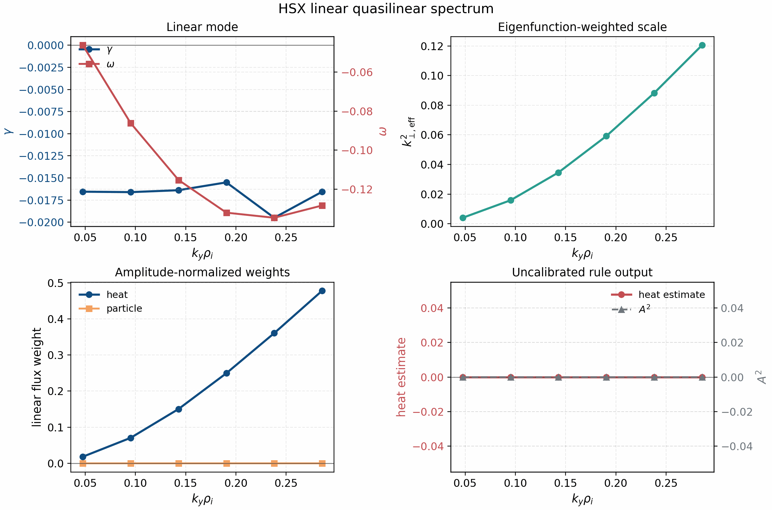
All scanned HSX branches in this short linear spectrum are stable under the
current gamma_floor = 0 mixing-length rule, so the uncalibrated saturated
heat-flux estimate is exactly zero even though the nonlinear HSX heat-flux
window is finite. This is a useful negative result: it shows that the current
one-constant mixing-length rule is not a transferable stellarator transport
model and that branch coverage/saturation physics must be improved before
absolute stellarator quasilinear-flux claims.
The combined Cyclone-train, Cyclone-Miller-holdout, and HSX-holdout report is generated with:
python tools/artifacts/plot_quasilinear_calibration.py report \
  --points docs/_static/quasilinear_cyclone_miller_train_holdout_points.json \
  --spectrum docs/_static/quasilinear_hsx_spectrum_scan.quasilinear_spectrum.csv \
  --nonlinear-summary docs/_static/nonlinear_hsx_gate_summary.json \
  --split holdout \
  --case hsx_nonlinear_window \
  --geometry hsx \
  --electron-model adiabatic \
  --fit-train-scale \
  --out docs/_static/quasilinear_hsx_train_holdout_report.json

python tools/artifacts/plot_quasilinear_calibration.py \
  --report docs/_static/quasilinear_hsx_train_holdout_report.json \
  --out docs/_static/quasilinear_hsx_train_holdout.png
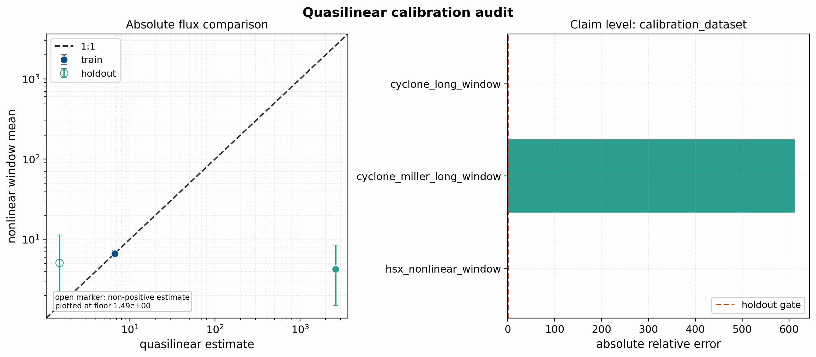
The report remains calibration_dataset and passed = false. In the
absolute-flux panel, open markers denote non-positive quasilinear estimates that
are plotted at the documented log-axis floor. The HSX point has a finite
nonlinear heat-flux window mean but zero current mixing-length prediction, so
the relative error is one by construction.
W7-X NetCDF nonlinear-window path
W7-X uses the same calibration machinery, but the tracked nonlinear window is a
runtime NetCDF file rather than a diagnostics CSV. The report builder therefore
uses the NetCDF ingestion path described above. A reproducible linear
quasilinear spectrum should be generated from a VMEC source, not from an
ignored local tools_out/*.eik.nc file:
cd examples/vmec
vmex input.nfp3_QI_fixed_resolution_final
cd ../..
gkx scan-runtime-linear \
  --config examples/linear/non-axisymmetric/runtime_w7x_linear_quasilinear_vmec.toml \
  --ky-values 0.047619047619047616,0.09523809523809523,0.14285714285714285,0.19047619047619047,0.23809523809523808,0.2857142857142857 \
  --Nl 4 --Nm 8 --solver time --dt 0.005 --steps 400 \
  --quasilinear \
  --out docs/_static/quasilinear_w7x_spectrum_scan \
  --no-progress
The bundled command above regenerates the demo spectrum from the shipped QI
VMEC input deck after vmex creates
examples/vmec/wout_nfp3_QI_fixed_resolution_final.nc. Exact W7-X
validation should use the same TOML with --vmec-file pointing to the
machine-specific benchmark WOUT; the benchmark WOUT itself is not shipped in
Git.
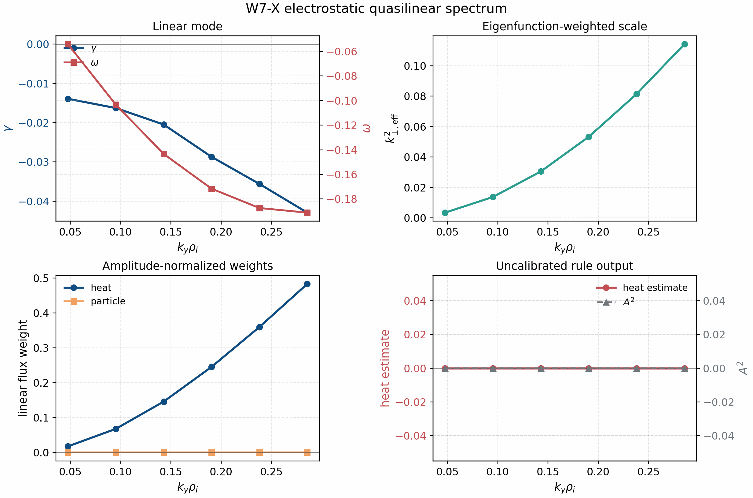
All six short-window W7-X linear branches in the tracked electrostatic
adiabatic-electron scan are stable under the current gamma_floor = 0 rule.
As for HSX, this makes the uncalibrated saturated mixing-length flux zero even
though the nonlinear heat-flux window is finite. The W7-X nonlinear NetCDF
window is added to the same train/holdout report with:
python tools/artifacts/plot_quasilinear_calibration.py report \
  --points docs/_static/quasilinear_cyclone_miller_train_holdout_points.json \
  --spectrum docs/_static/quasilinear_w7x_spectrum_scan.quasilinear_spectrum.csv \
  --nonlinear-summary docs/_static/nonlinear_w7x_gate_summary.json \
  --split holdout \
  --case w7x_nonlinear_window \
  --geometry w7x \
  --electron-model adiabatic \
  --fit-train-scale \
  --out docs/_static/quasilinear_w7x_train_holdout_report.json
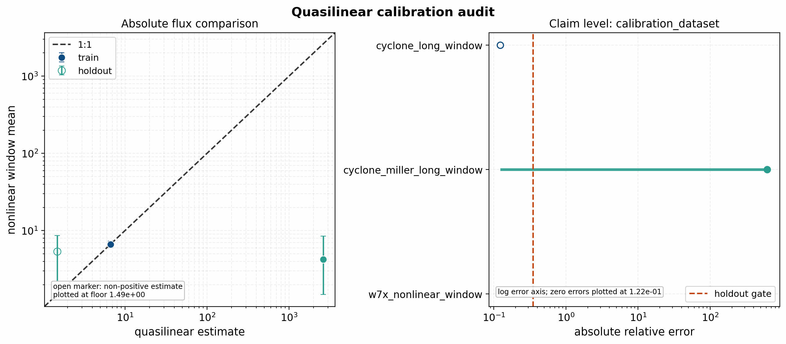
The report remains calibration_dataset and passed = false. The
Cyclone-fitted one-constant rule overpredicts Cyclone Miller, while the W7-X
stable branches underpredict the finite nonlinear window by construction. This
is retained as a negative absolute-flux result and should not be presented as a
validated W7-X transport model.
The manuscript-facing combined holdout panel now puts two training geometries (Cyclone and the admitted external-VMEC ITERModel case) together with nine held-out nonlinear windows: Cyclone Miller, HSX, W7-X, the admitted D-shaped external-VMEC case, the admitted up-down asymmetric external-VMEC case, the admitted circular external-VMEC case, the CTH-like and shaped-pressure external-VMEC cases admitted only by high-grid policies, the replicated QP external-VMEC case, and the replicated Solovev external-VMEC case.
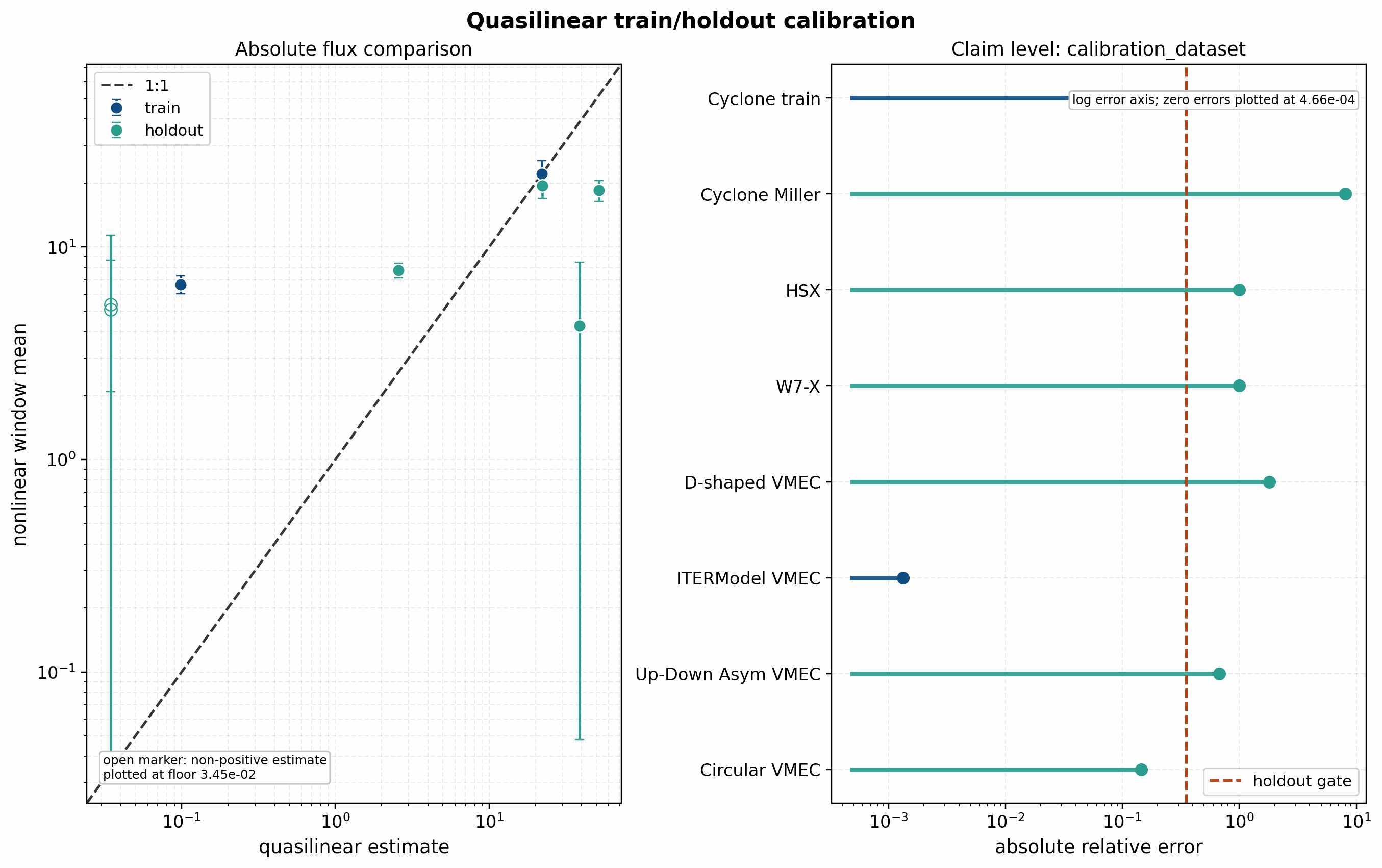
This combined report is also calibration_dataset and passed = false.
It is the clearest current figure for the absolute-flux story: one-constant
mixing length does not transfer across the present tokamak, stellarator, and
external-VMEC nonlinear windows. The fitted heat-flux scale uses only the two
training points and still leaves the ten holdouts at mean absolute relative
error about 6.49. The QP point is admitted by a seed/timestep replicated
t=250 ensemble, and the Solovev point is admitted by a repaired
n48/t250 seed/timestep ensemble with explicit 20% spread tolerance; the
QI point remains excluded as grid-sensitive negative evidence.
The external-VMEC points are included only after their high-grid convergence
gates passed or after a scoped high-grid admission gate passed: D-shaped
tokamak at t = 250, ITERModel at t = 350, up-down asymmetric tokamak
at t = 450, circular tokamak at t = 450, CTH-like external VMEC on the
t=[350,700] high-grid replicate window, and shaped-pressure external VMEC
on the t=[325,650] high-grid replicate window. The result is useful
precisely because it blocks premature absolute quasilinear transport claims
and motivates the next saturation-model sweep.
Saturation-rule sweep
The saturation-rule sweep compares three one-scalar intensity rules using the current 12-case train/holdout split: fit one multiplicative scale on the two training geometries and score the ten held-out windows. The tested rules are the current positive-growth mixing-length rule, the raw linear heat-flux weight, and an absolute-growth mixing-length diagnostic that gives stable branches nonzero intensity. The last rule is included only as a diagnostic stress test; it is not a validated physical saturation rule.
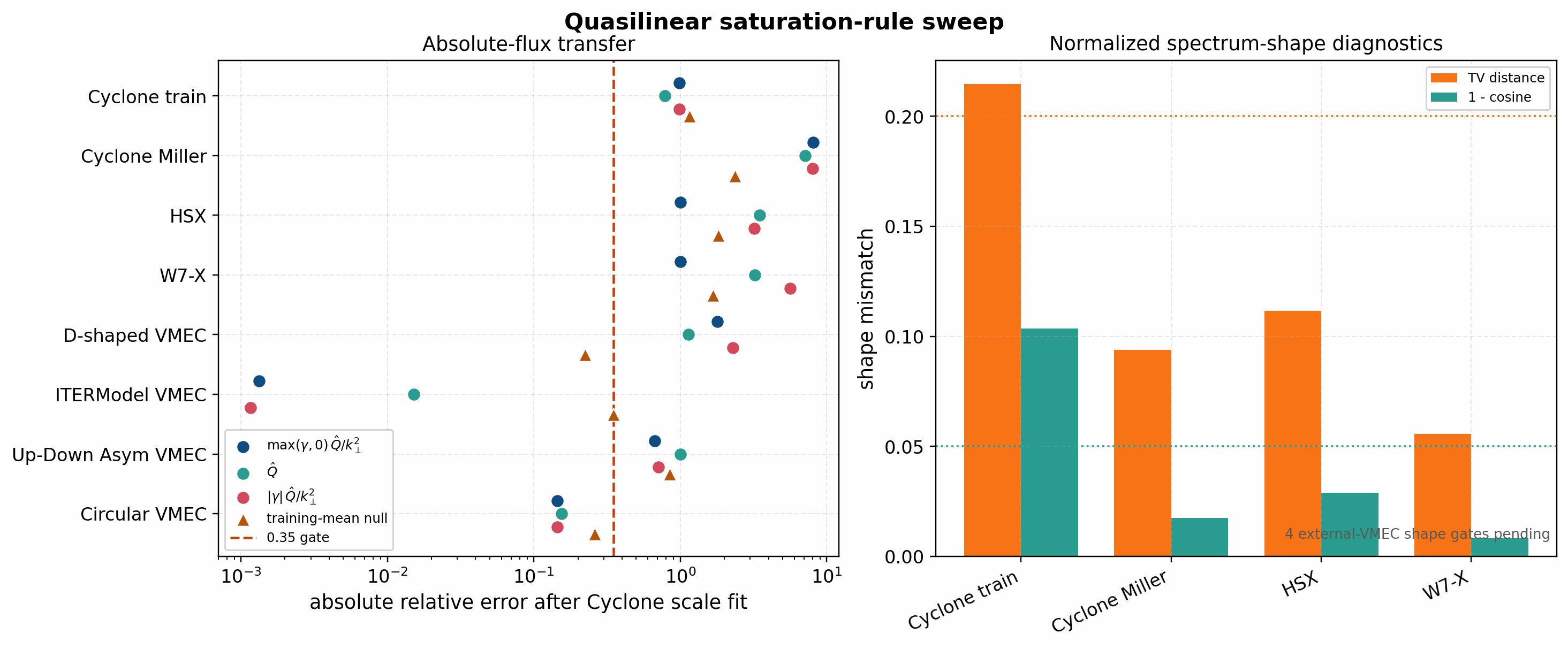
All tested one-scalar rules fail the held-out absolute-flux gate. On the
current 12-case sweep, the raw linear-weight rule is the least-bad simple rule
with holdout mean absolute relative error about 4.42. Positive-growth
mixing length is about 6.49, and the absolute-growth diagnostic is about
6.85. The figure also reports a training-mean null baseline; that null
gives holdout mean relative error about 1.80. It is not a quasilinear
model, but it is a necessary reviewer check: no calibrated saturation rule
should be promoted unless it beats this null baseline as well as the
linear-weight baseline. The JSON companion carries the same promotion_gate
and currently has no accepted rules. This narrows the next research task: the
admitted external-VMEC cases strengthen the negative transfer evidence, but
absolute-flux prediction still needs a richer saturation/intensity model than
any one-scalar fit tested here.
Shape-aware saturation diagnostic
The next diagnostic tests whether the missing information can be captured by a single low-dimensional shape envelope. It first forms the normalized nonlinear to quasilinear spectrum-shape ratio,
and fits a shared exponent with per-case intercepts,
The held-out prediction uses only training nonlinear shapes, training scalar
fluxes, and the held-out linear spectrum. It then fits the absolute heat-flux
scale on the training cases and scores the held-out nonlinear window. The
tracked figure uses --passed-shape-only for the exponent fit, so the
failed Cyclone shape gate does not contaminate the shape correction used for
the other geometries.
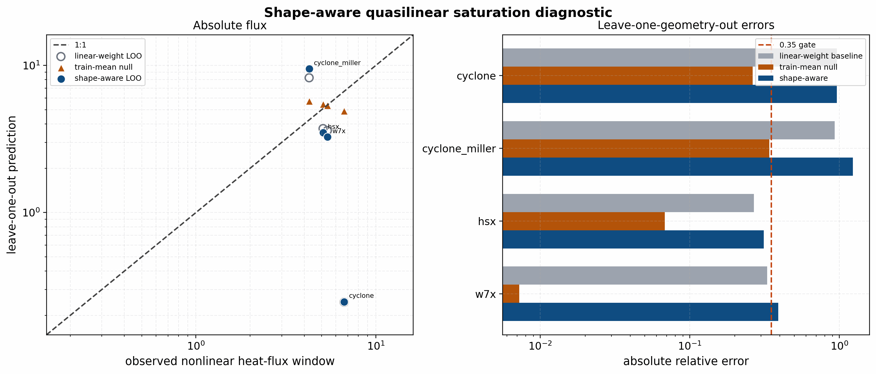
This is a useful negative result. The shape-aware power law gives mean
leave-one-geometry-out absolute relative error about 0.664, while the
linear-weight baseline gives about 0.624. Both fail the 0.35 absolute
transport gate, and the shape-aware model does not improve the mean held-out
score. The figure also includes a deliberately simple training-mean null
baseline; it gives mean relative error about 0.170 on this small dataset
because the archived nonlinear windows have similar absolute heat-flux levels.
That null baseline is not a quasilinear model, but it is the right reviewer
check: a calibrated saturation model should beat this baseline before being
used for absolute transport or optimization claims. This closes the
one-exponent saturation-envelope test and motivates a richer calibrated model
with branch/state features, uncertainty diagnostics, and electromagnetic
extensions. Its JSON companion also carries promotion_gate.passed = false
so the rejected model cannot be accidentally promoted by downstream scripts.
Candidate uncertainty gate
The candidate uncertainty gate adds prediction intervals to the same
leave-one-geometry-out protocol. For each held-out geometry, the candidate is
calibrated on the remaining cases, the training log-residuals define a
95% prediction interval, and the held-out point is scored against the
nonlinear heat-flux window. A candidate is promoted only if it:
passes the
0.35mean-relative transport gate;beats the training-mean null baseline;
beats the linear-weight baseline when it is a new non-baseline model;
reaches the interval-coverage gate;
passes candidate-specific eligibility checks such as minimum training-set size relative to the number of fitted parameters and matrix conditioning.
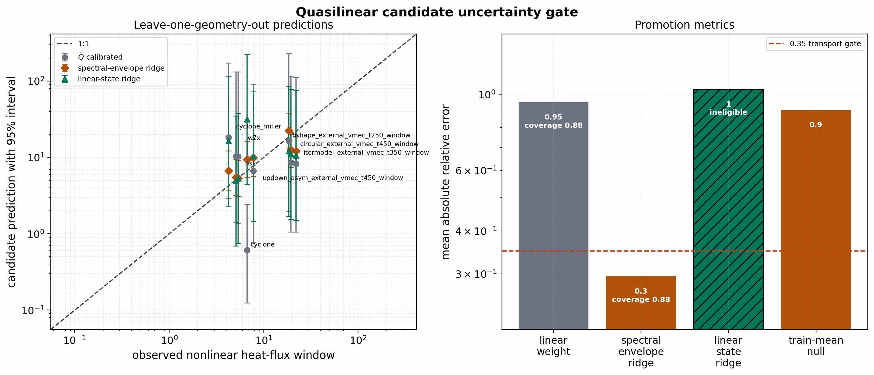
The stricter expanded ledger now includes the high-grid CTH-like,
shaped-pressure external-VMEC, replicated QP external-VMEC, and replicated
Solovev external-VMEC ensembles as held-out nonlinear points. On that 12-case
ledger, the reduced spectral_envelope_ridge candidate is still the best
candidate but is not accepted by the uncertainty gate: it reaches mean relative
error about 0.697 with interval coverage 11/12, above the 0.35
transport gate. The calibrated linear-weight baseline is worse (about
1.320), the training-mean null is about 1.171, and the broader
four-feature linear_state_ridge candidate is data-volume eligible but
performs poorly (mean relative error about 1.907). This is the intended research
posture after admitting tougher external-VMEC evidence: keep the small
spectrum-aware candidate as model-development signal, but not as an
uncertainty-validated flux predictor.
Residual-anatomy gate
The residual-anatomy artifact below asks a narrower reviewer-facing question: which cases make the current best reduced candidate fail, and are those errors coming from one geometry class or from the full portfolio? It consumes only the tracked uncertainty, screening, and saturation-rule JSON sidecars. It does not refit or promote a new model.
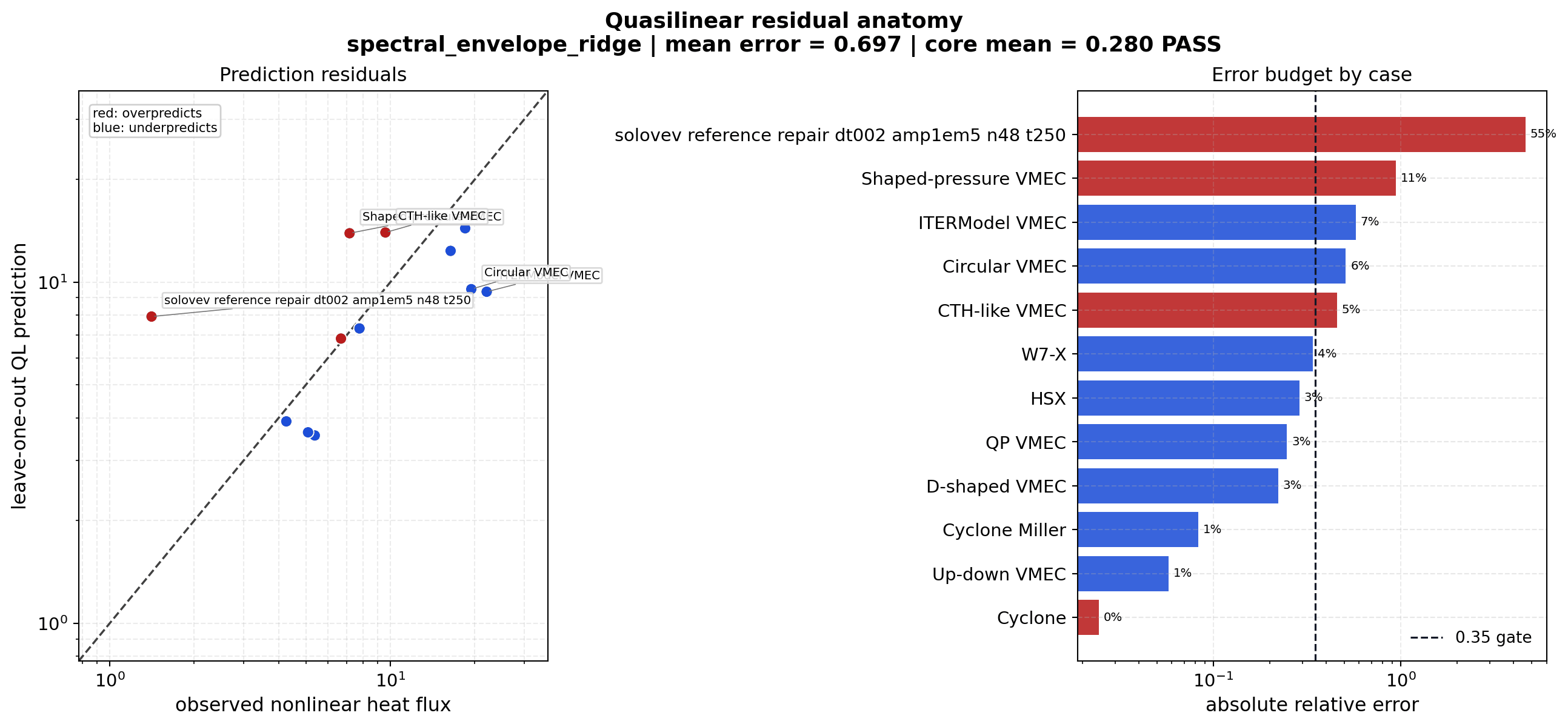
The current anatomy is specific enough to guide the next model-development
step. The replicated Solovev external-VMEC holdout is the largest residual, and
external axisymmetric VMEC cases contribute about 83% of the residual
budget for spectral_envelope_ridge. In contrast, the admitted HSX and W7-X
benchmarks remain materially less severe stress cases, with mean relative error
about 0.31 in this reduced candidate.
That split argues against a looser universal acceptance threshold: the next
absolute-flux attempt should keep this twelve-case ledger fixed and improve
the saturation physics enough to distinguish low-flux axisymmetric stress
cases, pressure shaping, and stellarator turbulence windows. Additional
holdout collection is not the active remedy for this tranche.
Regularization sensitivity audit
The near miss above is small enough that reviewer-facing documentation needs to
show it is not an artifact of one arbitrary ridge penalty. The regularization
audit below reruns the same leave-one-geometry-out spectral_envelope_ridge
fit across a ridge-penalty sweep and records the best admissible setting.
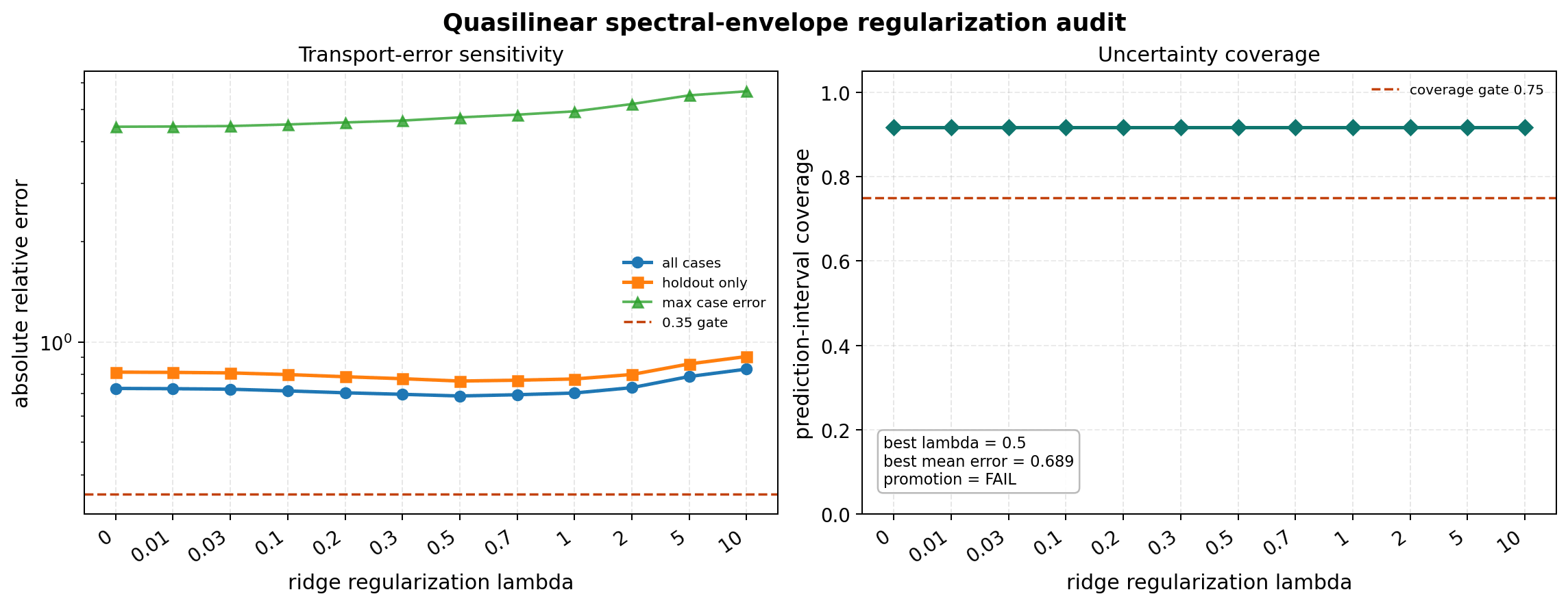
The best tracked penalty is lambda = 0.5. It gives full-ledger mean
relative error about 0.689, held-out mean relative error about 0.764,
and prediction-interval coverage 11/12. No tested penalty passes the
0.35 transport gate. The conclusion is therefore stable under this
regularization sweep: the spectral-envelope candidate is useful as a
model-development diagnostic, but not as an absolute heat-flux predictor.
Stellarator usefulness summary
The stellarator-focused summary below is generated from existing validation artifacts only; it does not refit a model or add any unvalidated nonlinear points. It compares the admitted HSX, W7-X, CTH-like, and shaped-pressure nonlinear windows against the current quasilinear candidates, then records the present status of the QA and QH optimization families.
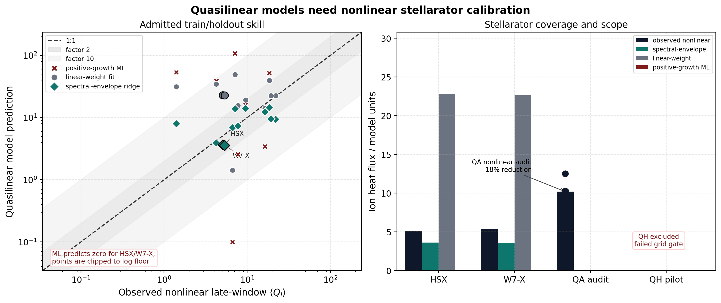
The result is intentionally mixed. For HSX and W7-X, the simple
positive-growth mixing-length rule predicts zero because the tracked short
linear branches are stable under gamma_floor = 0, while the admitted
nonlinear heat-flux windows are finite. That is a direct fail for this simple
absolute-flux proxy. The raw linear-weight fit is nonzero but overpredicts
both stellarator holdouts by roughly a factor of four. The shaped-pressure
holdout is the opposite stress test: the one-scalar positive-growth rule
overpredicts it strongly. The reduced spectral_envelope_ridge candidate is
closer for HSX and W7-X and remains the best current scoped model-development
candidate, but it fails the current 12-case transport and rank-screening gates
and is not a runtime saturation law or universal stellarator transport model.
This behavior is consistent with the literature rather than surprising. Modern tokamak quasilinear transport models separate linear flux weights from an empirical or theory-assisted saturation rule [Stephens21] [Parker23] [Staebler24]. Stellarators add additional sensitivity because the nonlinear state can involve many subdominant and stable eigenmodes [Pueschel16], energy transfer to damped modes [Hegna18], and zonal-flow dynamics [Tiwari25]. The QHS/QAS comparison in [McKinney19] likewise emphasizes that linear growth rates alone are a weak proxy for saturated heat flux across quasi-symmetric stellarators. The GKX conclusion is therefore: quasilinear metrics are useful for exploratory screening, differentiable optimization research, and model-development figures, but reliable absolute nonlinear heat-flux prediction for QA, QH, W7-X, and HSX requires more matched nonlinear holdouts and a richer saturation theory calibrated against those holdouts.
Screening and rank-correlation gate
Absolute flux is not the only useful model-development target. For optimization and early design screening, a calibrated quasilinear candidate can still be useful if it ranks geometries in approximately the same order as the nonlinear late-window heat flux. The screening gate below therefore scores each candidate with both absolute-error and rank/correlation metrics, while keeping absolute flux promotion disabled unless the stricter holdout-promotion requirements also pass.
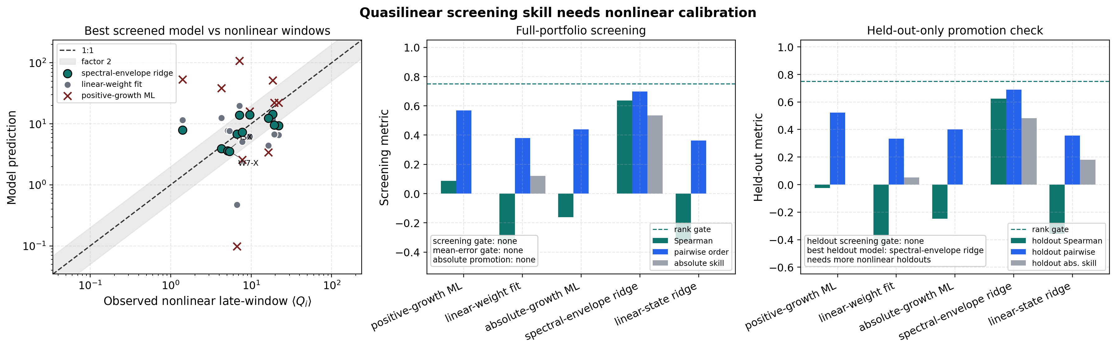
The current result is stronger than the simple one-constant story but still
properly scoped. On the expanded 12-case electrostatic portfolio, no model
passes both the full and held-out rank/correlation screening gates. The best
candidate remains spectral_envelope_ridge with full-portfolio Spearman
correlation about 0.636 and pairwise order accuracy about 0.697;
held-out-only Spearman is about 0.624 with pairwise order accuracy about
0.689. Its held-out mean relative error is about 0.777, above the
0.35 absolute-error gate. The simple positive-growth mixing-length rule,
raw linear-weight fit, absolute-growth diagnostic, and broader linear-state
ridge do not pass the screening gate either. This supports using the
spectral-envelope candidate as a model-development diagnostic only, not as a
runtime/TOML absolute-flux predictor, promoted rank screener, or universal
stellarator saturation law.
The next calibration step is not a looser threshold; it is additional
independent, replicated, post-transient nonlinear holdouts.
All three model-development reports above now carry an input_validation
block. It is generated from the nonlinear summary gates before model fitting,
so these figures can only be regenerated from nonlinear windows that already
passed their validation gates. This is intentionally stricter than a finite-run
check: exploratory external-VMEC pilots remain useful for planning, but they
cannot enter these quasilinear model diagnostics until their convergence and
validation gates pass.
Dataset-sufficiency gate
The current electrostatic-compatible dataset is large enough to reject simple saturation-rule hypotheses and to promote a bounded richer candidate, but it is still not large enough to justify every higher-parameter model class. The dataset-sufficiency gate makes that reviewer-facing scope explicit before any model fit is attempted. It requires:
nonlinear input summaries that have already passed their validation gates;
at least six electrostatic-compatible calibration cases;
at least two explicit training geometries and three held-out geometries;
enough leave-one-out training cases per fitted parameter for richer candidates;
passed downstream saturation-rule and uncertainty/skill gates.
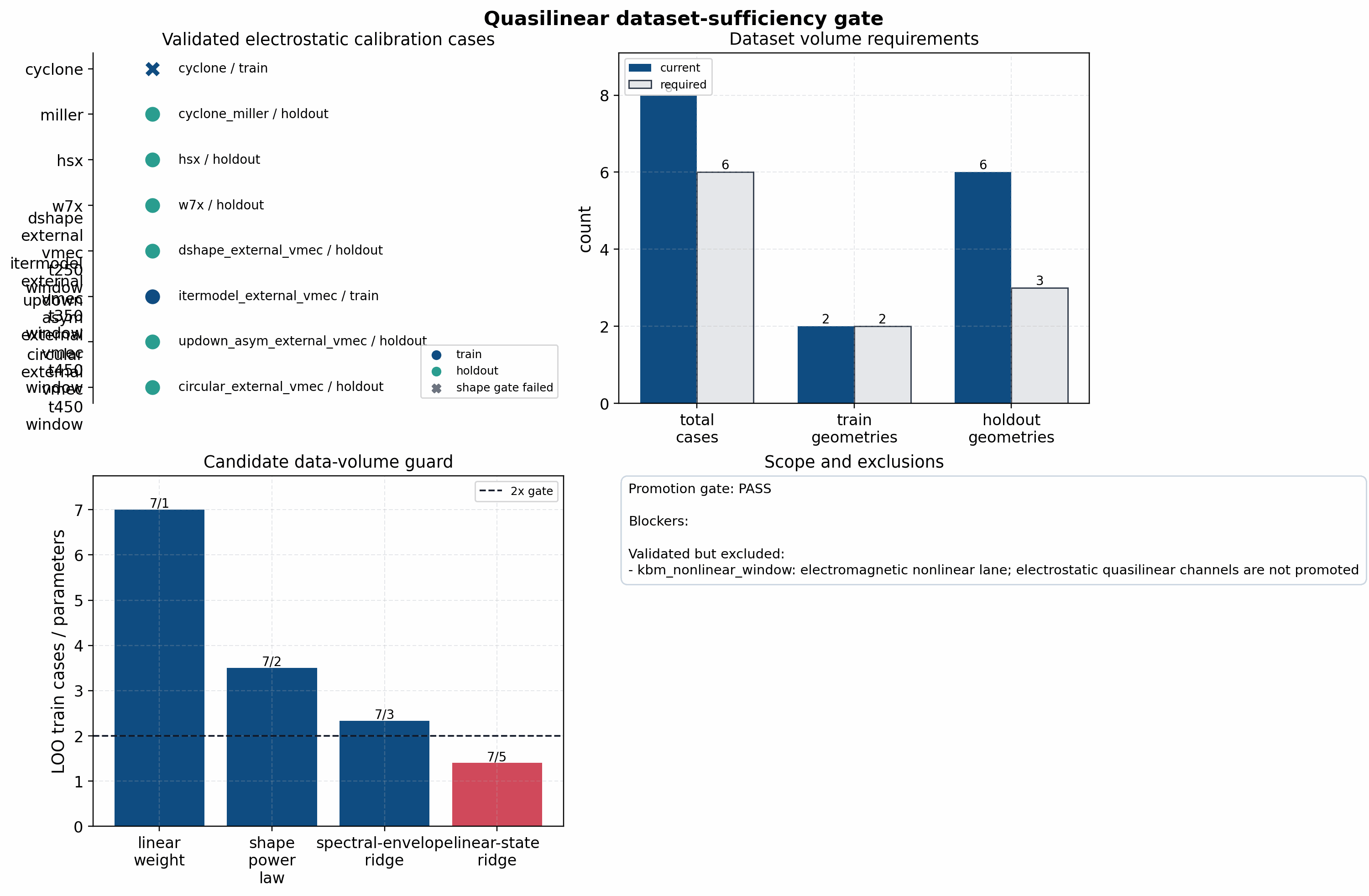
The tracked gate now fails closed on downstream candidate skill for the
expanded candidate-model dataset. There are now twelve admitted
electrostatic-compatible cases, two explicit training geometries, and nine
held-out geometries. That is enough data volume for the one-parameter
linear-weight candidate, the two-parameter shape-power-law candidate, the
three-parameter spectral_envelope_ridge candidate, and the five-parameter
linear_state_ridge model at the configured leave-one-out train-to-parameter
threshold. However, the sufficiency artifact still fails closed because the
downstream candidate-skill gate is not passed on the expanded ledger. KBM is
still listed as a validated but excluded nonlinear case because the present
quasilinear diagnostics are electrostatic; electromagnetic quasilinear
field-channel normalization and calibration remain separate future work.
Model-selection status
The model-selection status combines the dataset-sufficiency gate, candidate uncertainty gate, and all tracked train/holdout calibration reports into one claim-boundary artifact. It is intentionally not another fit. It answers the reviewer-facing question: is there a positive scoped model-selection result, and are we still avoiding an absolute-flux overclaim?
The current status does not pass after the CTH-like and shaped-pressure
holdouts are admitted. The spectral_envelope_ridge candidate has
leave-one-geometry-out mean relative error about 0.697 and interval
coverage 11/12. It beats the calibrated linear-weight baseline (1.320)
but is above the 0.35 transport gate and does not pass the downstream
candidate-skill gate. The model-selection status
therefore records blockers dataset_sufficiency_passed,
candidate_uncertainty_passed, required_candidate_accepted, and
required_candidate_transport_error. This is a useful negative update for
the manuscript: it keeps the reduced-model ledger fail-closed, not as a
runtime/TOML absolute-flux predictor, universal saturation rule, promoted rank
screener, or nonlinear turbulence-gradient optimization claim.
The companion claim-boundary artifact
docs/_static/nonlinear_turbulence_gradient_evidence_status.json is
deliberately stricter: it records that replicated long-window transport
evidence is present, while the current nonlinear-gradient artifact is a
long-window production candidate that still fails closed on plus-state
transport-window spread and propagated gradient uncertainty. The current
tracked artifact is the QA/ESS ZBS(1,0) 7.5% bracket: all twelve
t=900 nonlinear outputs pass the t=[450,900] output gates, the response
is resolved (response_fraction = 0.0319), and the finite-difference
bracket is local (fd_asymmetry_rel = 0.044), but the plus ensemble spread
is 0.196 > 0.15 and gradient_uncertainty_rel = 1.81 > 0.5. It is
therefore not promoted as production turbulence-gradient evidence.
Holdout-gap report
The holdout-gap report is the reviewer-facing companion to the model-selection status. It answers a different question: which currently tracked nonlinear windows are admitted, which candidate windows are excluded, and what exact data product is needed before absolute-flux promotion can be reconsidered?
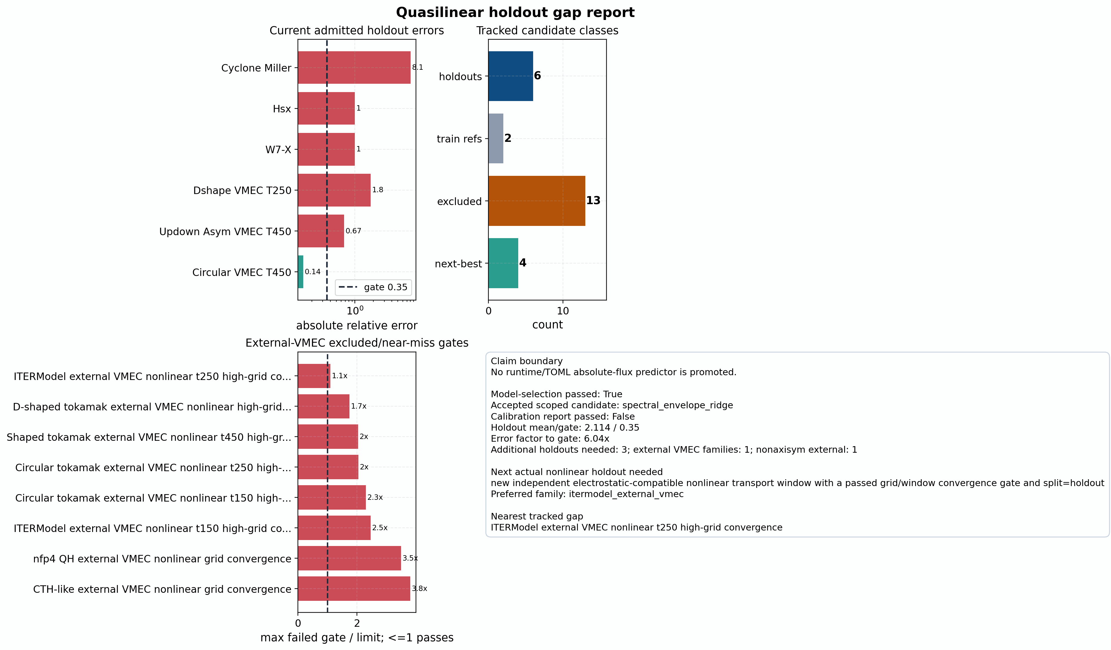
The current report admits ten holdouts and two training references, but it
keeps absolute_flux_promoted = false because the aggregate held-out
absolute-flux error remains about 6.49 against the 0.35 gate. The
spectral_envelope_ridge candidate remains the best reduced candidate, but
its uncertainty/model-selection gate is not accepted. Its mean
leave-one-geometry-out relative error is about 0.697 on the expanded
ledger, above the 0.35 gate, and that number is not a saturated
absolute-flux promotion because it comes from the candidate-selection
uncertainty report rather than a passed absolute train/holdout calibration
artifact.
The JSON sidecar now carries explicit
absolute_flux_promotion_requirements and
screening_promotion_requirements blocks. For the current frozen artifacts,
no full-portfolio or held-out-only screening model is accepted after adding the
shaped-pressure holdout, and the independent-holdout-count blocker is closed, but screening promotion
still fails the rank/correlation and transport-error gates. The external-VMEC
family coverage gates are satisfied by CTH-like and shaped-pressure high-grid
admissions, but these are evidence requirements, not automatic promotion
criteria; any future model must still pass the held-out transport-error gate,
prediction interval/skill gates, and provenance checks on the same frozen case
ledger.
The report now tracks the shaped-tokamak-pressure reference as a scoped
high-grid admission rather than as an excluded failed-family candidate. The
full n48/n64/n80, t = 450, dt = 0.04 ladder fails only because the
coarse n48 trace is not converged: the common/least pairwise heat-flux
shift is about 0.469, above the 0.15 gate. The retained n64/n80
pair passes at both t = 450 and t = 650 with common-window relative
differences about 0.0789 and 0.0983. The high-grid time-horizon gate
also passes, with common/least changes about 0.0418/0.1237, and the
n80 seed/timestep ensemble passes on t=[325,650] with mean heat flux
7.16, mean-relative spread 0.0939, and combined SEM/mean 0.0463.
The dedicated high-grid admission sidecar therefore admits this case only
under coarse-grid exclusion. It is not a full n48/n64/n80 convergence claim
and not an absolute-flux promotion.
The added holdout makes the quasilinear model-development ledger more honest
and more difficult. The portfolio now contains 12 electrostatic-compatible cases with ten
holdouts. Positive-growth mixing-length transfer has holdout mean relative
error about 6.49 against the 0.35 transport gate; the best
spectral-envelope candidate has leave-one-geometry-out mean error about
0.697 and does not pass the full or held-out rank/correlation screening
gates. Absolute-flux promotion remains blocked by transport error and
screening failure, not by missing holdout count.
The matched strict QA full-sweep audit is also deliberately excluded from this
calibration ledger. The office campaign completed the raw baseline, linear-
growth optimized, quasilinear-optimized, and nonlinear-window-optimized runs,
but the postprocess requested the strict t=[1100,1500] admission window
while every harvested trace ends near t=400. The replicated ensemble
artifacts
docs/_static/optimized_equilibrium_replicates/vmec_qa_full_sweep_*_ensemble_gate.json
therefore have n_finite_means = 0, and the matched comparison artifacts
docs/_static/qa_strict_baseline_to_*_strict_baseline.json are
passed = false with no computable relative reduction. These outputs are
useful negative audit evidence and a command-generation regression test; they
are not nonlinear holdouts, are not used to refit the quasilinear calibration,
and do not change the screening/absolute-flux promotion status above.
External-VMEC holdout results
The tracked evidence keeps completed validation results rather than a generated
campaign planner. ITERModel and shaped-pressure cases are already represented,
and replaying them would not add independent holdout leverage. The modified QH
ladder remains negative evidence: its weak finite branch
(gamma = 0.022949 at ky = 0.4762) was followed to t=700 on
n64/n80 with dt=0.04, but the common- and least-window heat-flux
differences, about 0.349 and 0.367, fail the relaxed 20% gate. The
independent Solovev seed/timestep ensemble passes with mean heat flux 1.409
and relative spread 0.1599. These high-grid admission and ensemble JSON
artifacts are calibration evidence, not a universal absolute-flux promotion.
VMEC equilibrium portfolio for future holdouts
The next quasilinear promotion attempt needs more matched nonlinear holdout
windows, not more fit parameters. The local vmex checkout includes a
useful portfolio of small VMEC equilibria that can seed those future linear
scans and nonlinear validation runs without adding the VMEC files to the
GKX repository. The inventory tool records file sizes, checksums,
nfp, resolution, aspect ratio, edge rotational transform, beta, and a
selection score for follow-up cases.
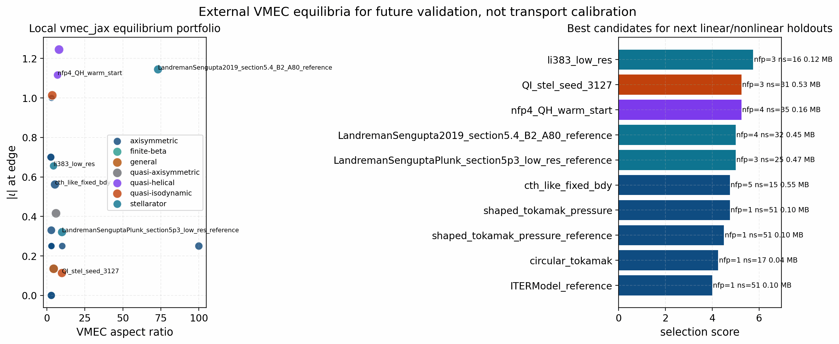
The current inventory finds 11 local VMEC equilibria. The best immediate
linear/nonlinear holdout candidates are wout_li383_low_res.nc,
wout_QI_stel_seed_3127.nc, wout_nfp4_QH_warm_start.nc,
wout_cth_like_fixed_bdy.nc,
wout_shaped_tokamak_pressure.nc, wout_circular_tokamak.nc,
wout_DSHAPE.nc, and wout_purely_toroidal_field.nc. The
wout_LandremanPaul2021_QA_lowres.nc fixture is deliberately deferred by the
inventory gate because its VMEC reference scale metadata are degenerate
(Aminor_p = Rmajor_p = aspect = volume = 0), which is not a valid input to
the current VMEC-to-EIK runtime path.
The first bounded smoke scans use ky = 0.10, 0.20, Nl = 2,
Nm = 4, dt = 0.005, and 80 explicit time steps to check only that
the geometry path, linear solve, and quasilinear-feature writer are finite.
They are intentionally short and should not be interpreted as optimized
physics scans:
VMEC fixture |
smoke result |
sampled growth rates |
|---|---|---|
|
finite stable branches |
|
|
finite stable branches |
|
|
finite stable branches |
|
|
finite stable branches |
|
These are not accepted quasilinear transport calibration points yet. Each candidate must first get a reproducible production-resolution GKX linear quasilinear scan, a matched nonlinear heat-flux window, and a passed nonlinear comparison/physics gate before entering the leave-one-out calibration reports above.
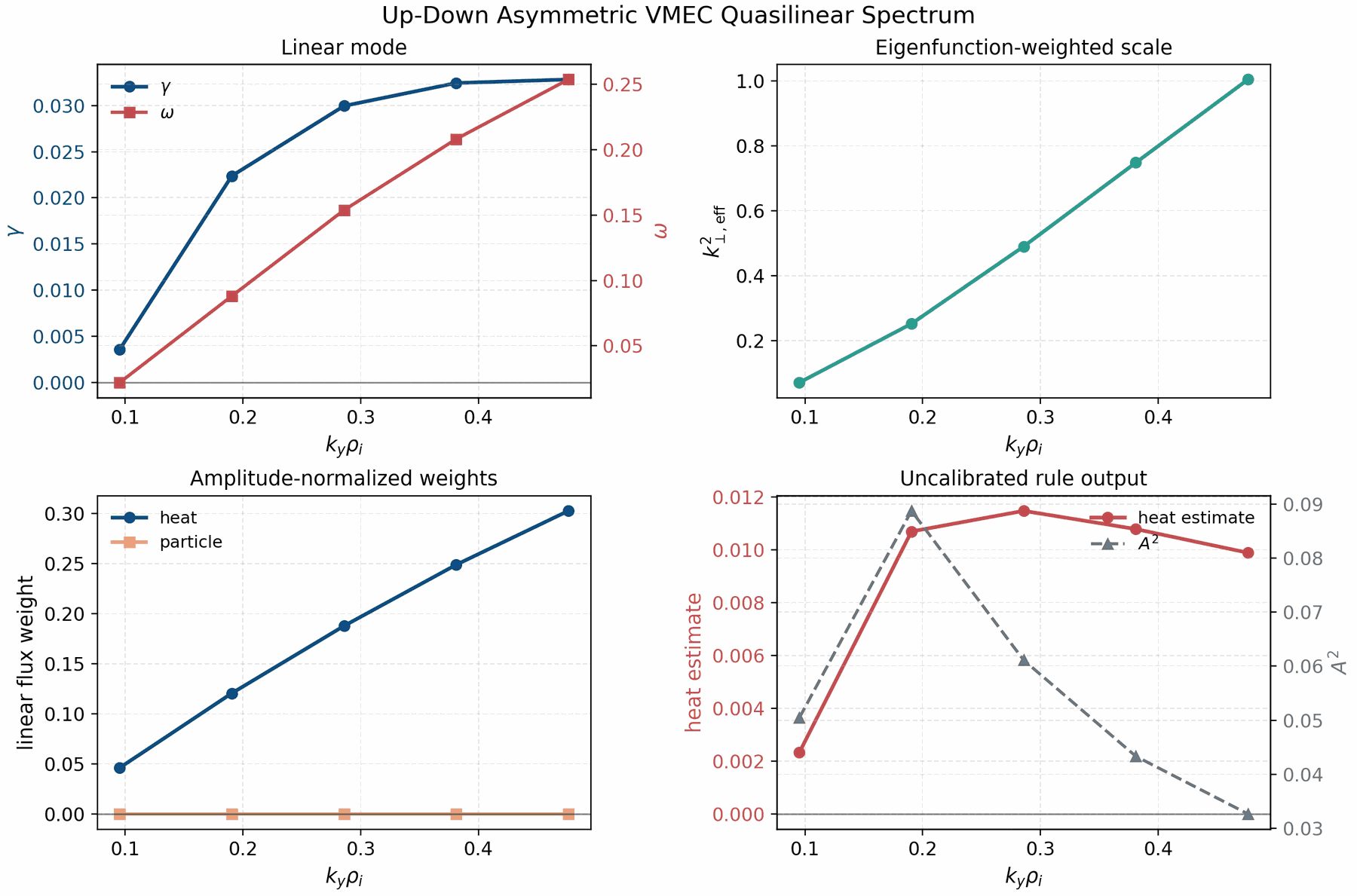
The first full-ky follow-up kept the same W7-X-style VMEC runtime TOML but
used Nl = 4, Nm = 8, and 400 explicit time steps over the six-point
stellarator ky grid used elsewhere in this documentation. Li383 remains
stable over that short linear scan, with gamma decreasing from about
-0.022 to -0.078. The shaped-tokamak fixture is also stable over the
same grid, with gamma increasing from about -0.080 to -0.0186 but
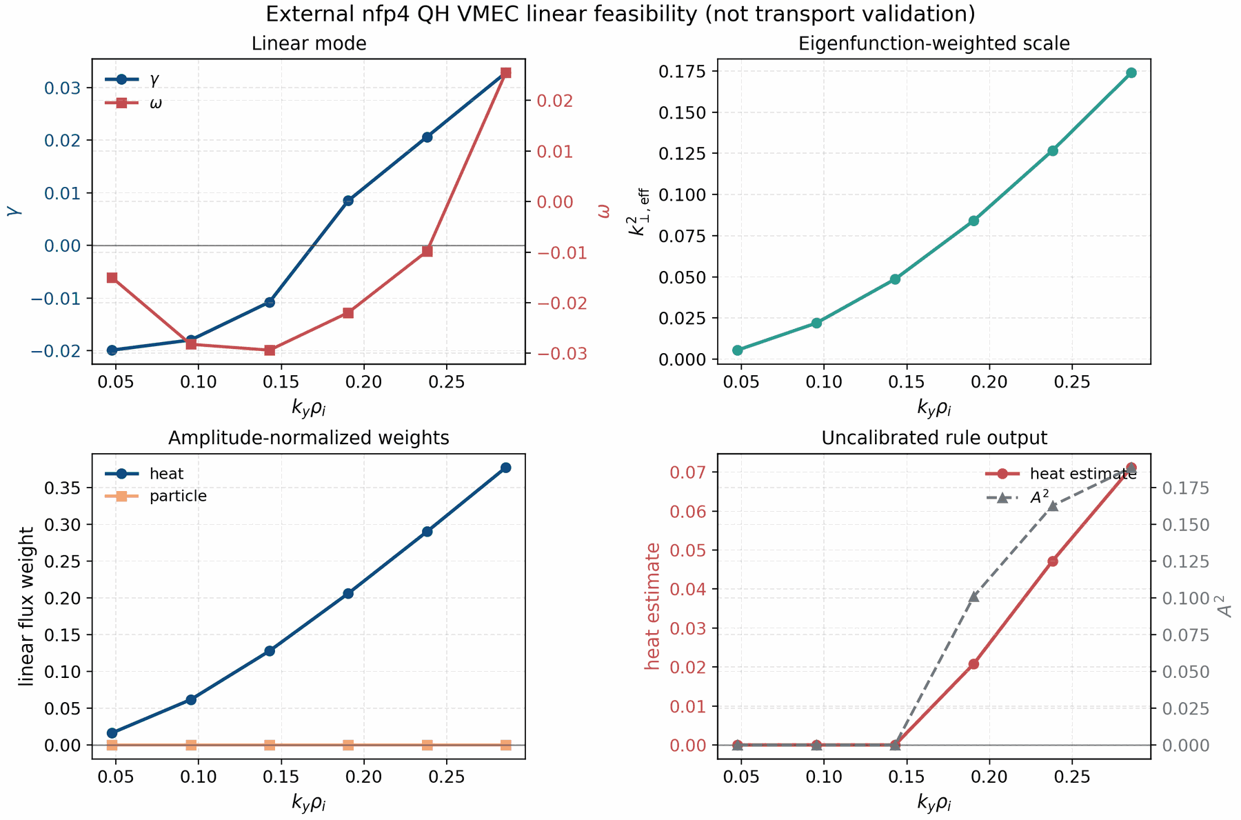
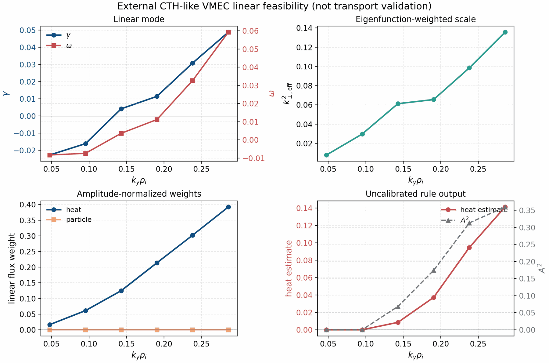
not crossing zero. The nfp4 QH and CTH-like fixtures are more useful for the
next validation lane: QH reaches gamma = 0.0328 at ky = 0.2857, while
CTH-like reaches gamma = 0.0488 at the same sampled ky. The figures
below are still linear-feasibility artifacts only; they motivate matched
nonlinear windows but do not validate an absolute quasilinear saturation rule.
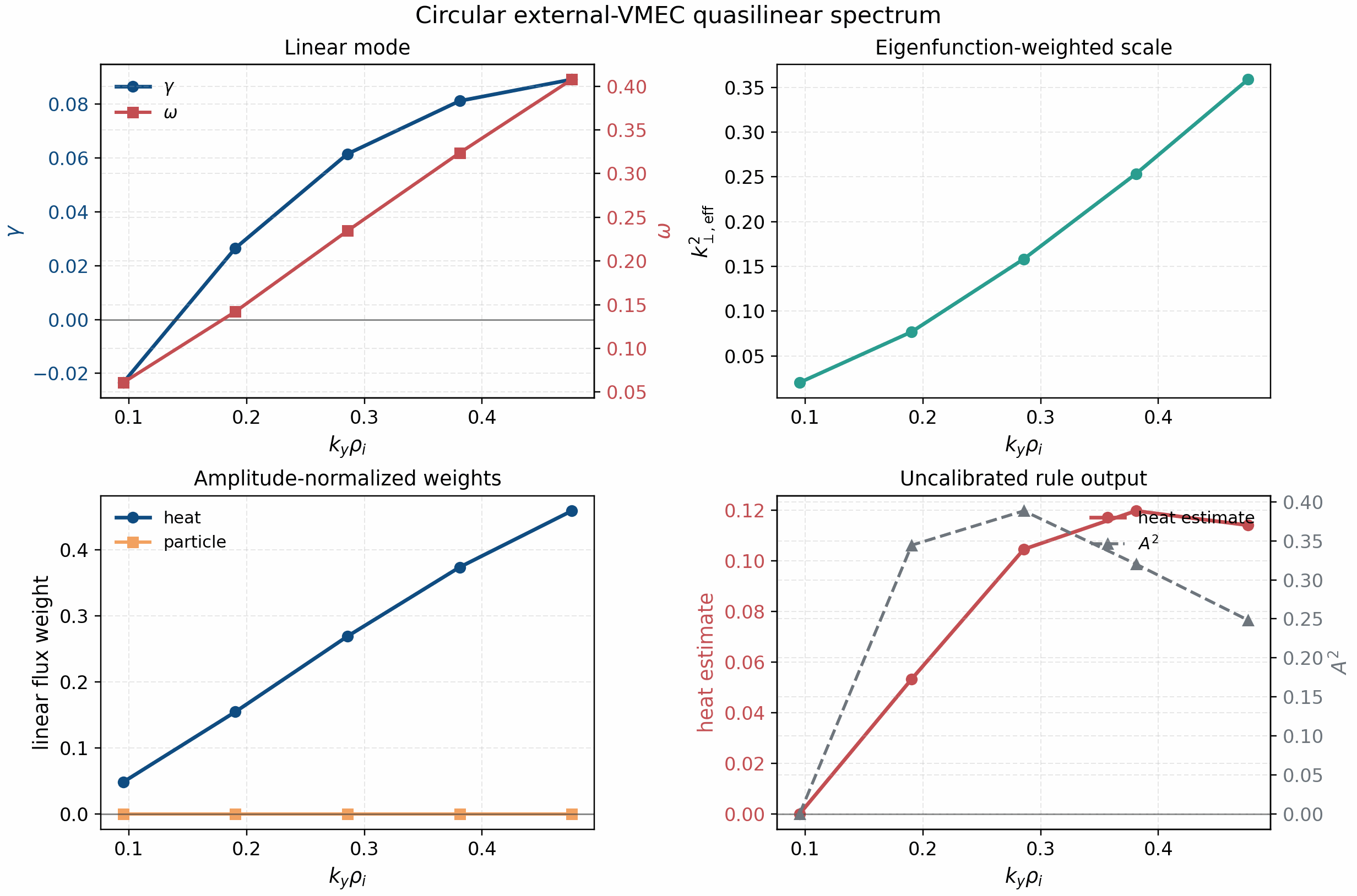
The QH convergence failure triggered a broader candidate screen before any
additional nonlinear promotion. The five-point screen uses
ky = 0.095, 0.190, 0.286, 0.381, 0.476, Nx = Ny = 48, Nz = 32,
Nl = 4, Nm = 8, and 400 explicit RK4 steps. Among the finite
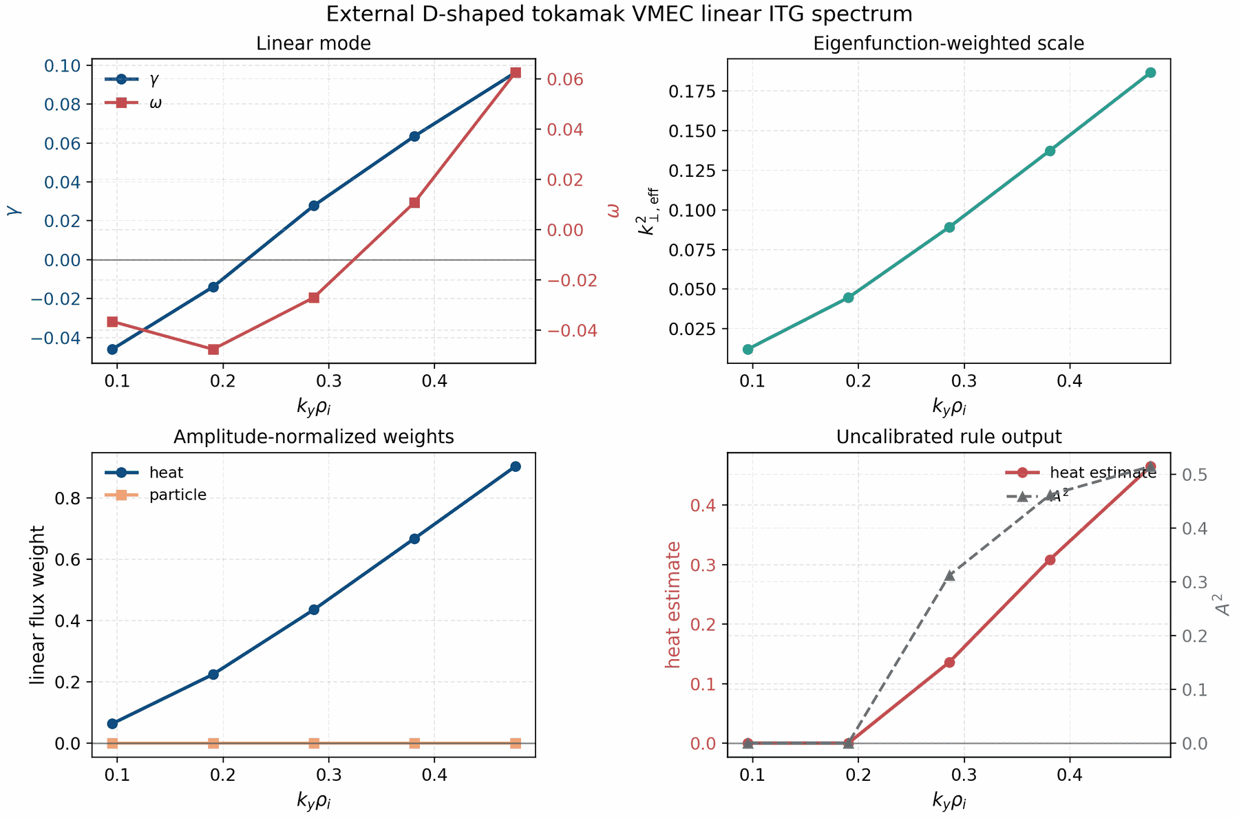
external-VMEC candidates, wout_DSHAPE.nc is the strongest unstable branch
with gamma = 0.096 at ky = 0.476. Circular tokamak and ITER-model
fixtures are close behind, while QI/QA/QH reference fixtures are stable or fail
the current geometry screen. The screen output is tracked as
docs/_static/external_vmec_candidate_linear_screen.csv.
The refreshed local portfolio adds three explicit outcomes to that screen. The
finite-beta wout_li383_low_res.nc branch stays stable over
ky = 0.095 to 0.476 under the same adiabatic-electron ITG screen. The
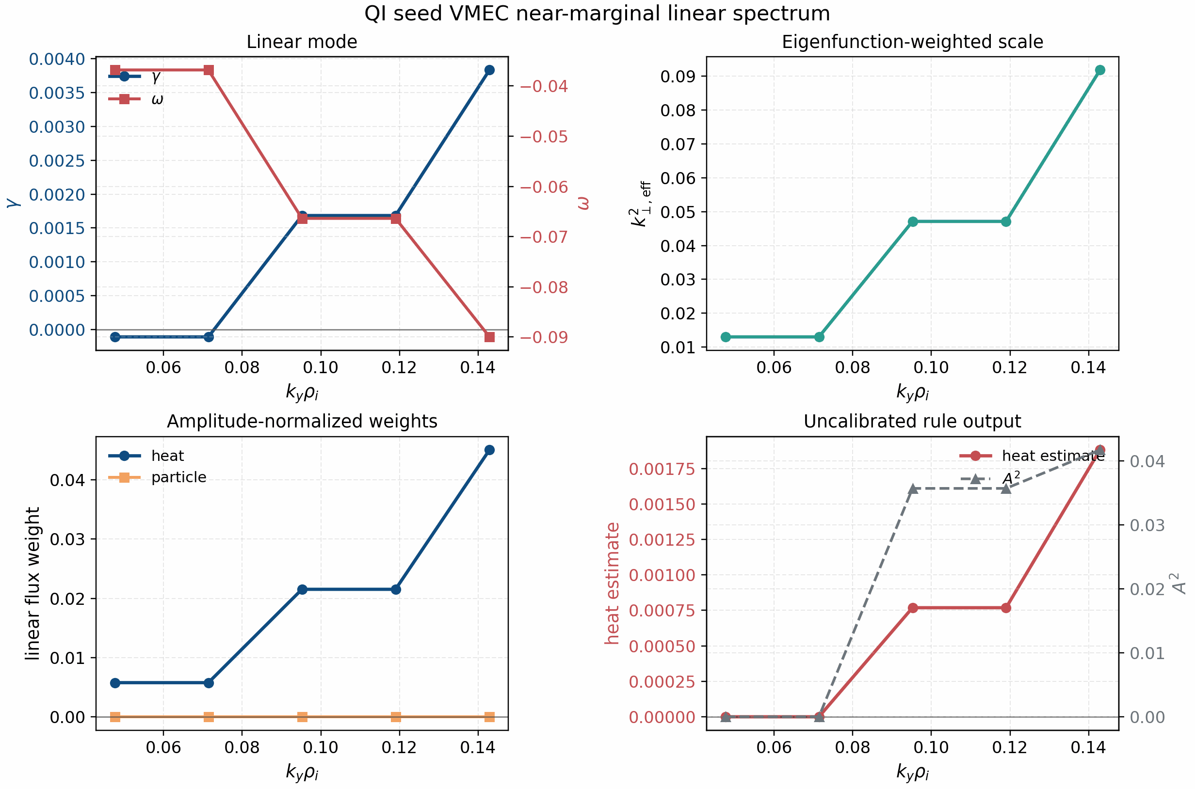
new wout_QI_stel_seed_3127.nc branch is finite and only weakly unstable:
the refined low-ky scan peaks at gamma≈3.8e-3 near ky≈0.143, and a
Krylov check confirms the lowest-ky branch remains near marginality. The
current runbook therefore treats this as QI/seed-robust feasibility evidence,
not as a nonlinear transport launch target. A separate
wout_basic_non_stellsym_simsopt.nc attempt fails the present VMEC flux-tube
cut contract before time integration, so it is tracked as a geometry-contract
failure rather than a physics result.
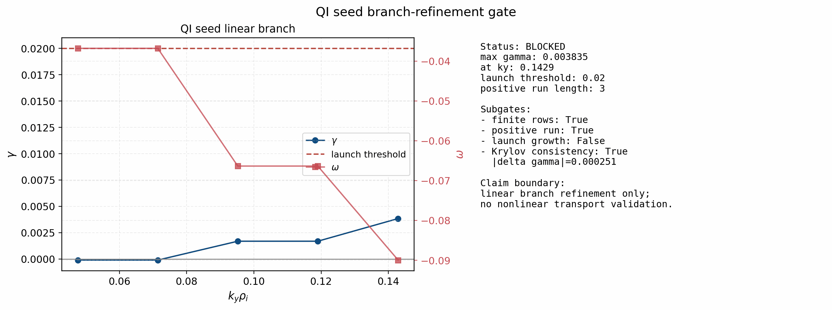
The companion branch-refinement gate compares the same time-propagated branch
with a Krylov check at the lowest unstable sampled mode. Finite rows,
contiguous positive low-ky support, and Krylov consistency pass, but the
launch-growth subgate fails because max(gamma)≈3.8e-3 is below the
0.02 nonlinear-launch threshold. This is the intended outcome: the result
is useful QI branch-continuation evidence, not a nonlinear transport validation
or absolute-flux calibration point.
Solved VMEC optimization outputs use the same launch discipline. The screen
consumes runtime linear-scan spectra from solved vmex WOUTs and
blocks nonlinear launches unless growth, metric, and heat-flux weights are all
finite and launchable. The tracked screen artifact is
docs/_static/vmec_optimization_candidate_screen_gate.json.
The current four-case CPU screen is fail-closed: qa_nfp2 is marginal,
qh_nfp3/qp_nfp4 are stable, and qp_nfp3 is rejected despite large
fitted growth because sampled effective k_perp^2 is non-positive. This is
candidate triage, not nonlinear transport validation.
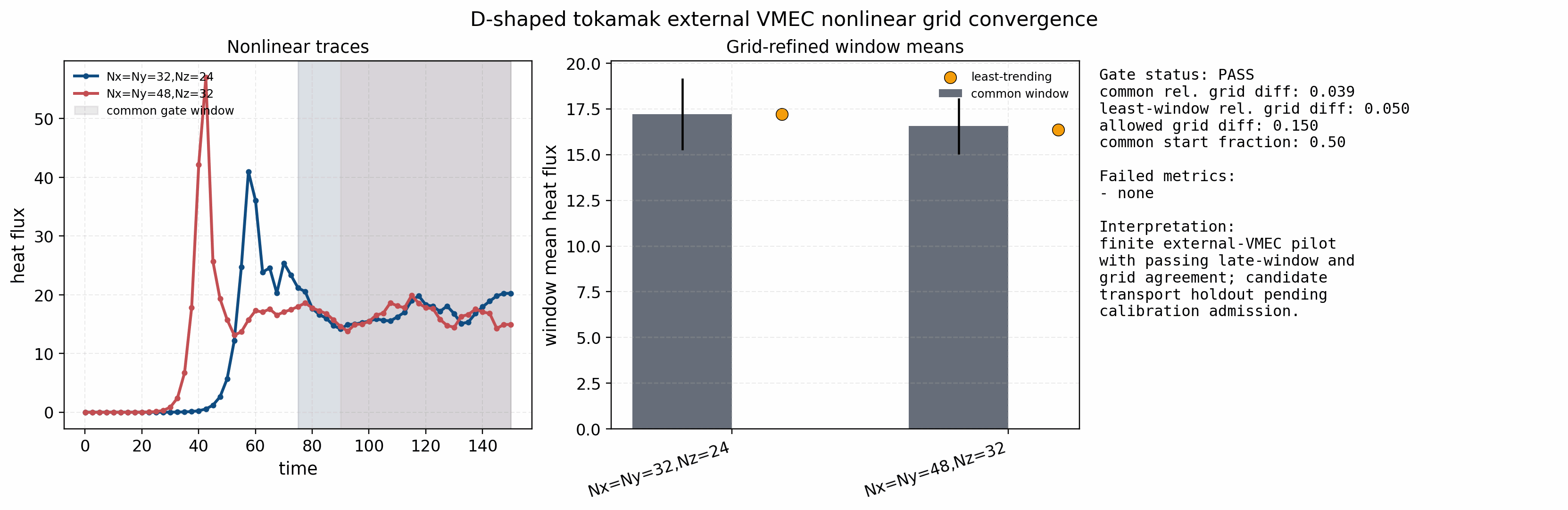
D-shaped tokamak nonlinear pilots were then run on the office GPUs with the
same ITG/adiabatic-electron physics as the QH and CTH-like pilots. The
t = 150 low-to-mid-grid gate passes immediately: Nx = Ny = 32,
Nz = 24 and Nx = Ny = 48, Nz = 32 differ by only 0.039 on the
common late-window mean and 0.050 on the least-trending-window mean. The
t = 150 mid-to-high-grid gate is close but not acceptable, with
0.201 common-window and 0.262 least-window relative differences. This
is exactly why the time-window check is required before promoting a run.
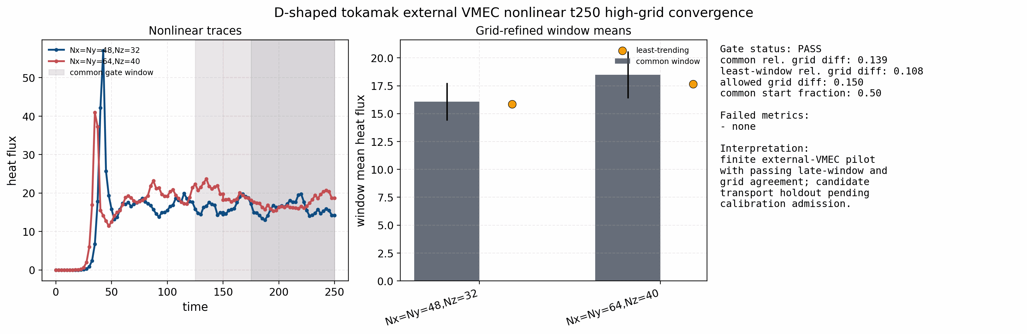
Extending the 48x48x32 and 64x64x40 runs from t = 150 to
t = 250 closes the gate. The common-window means are about 16.1 and
18.5 with symmetric relative difference 0.139; the independently
selected least-trending-window means are about 15.9 and 17.7 with
relative difference 0.108. Both are below the 0.15 threshold, and the
trend/CV/sample-count gates also pass. D-shaped tokamak is therefore the first
external-VMEC nonlinear transport holdout from this campaign admitted into the
quasilinear calibration report. Admission does not promote the current
absolute-flux model: the Cyclone-trained one-constant mixing-length estimate
overpredicts this D-shaped holdout by about two orders of magnitude.
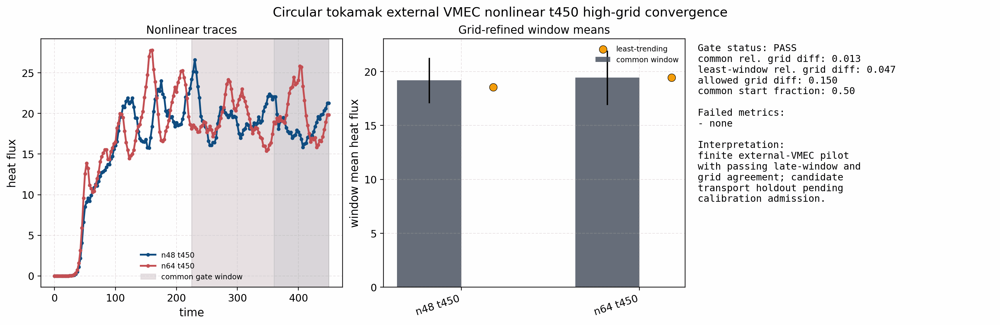
The circular-tokamak follow-up is now a useful example of why bounded
extension ladders must be explicit. At t = 150 the 48x48x32 to
64x64x40 pair had excellent grid agreement but still failed the common and
least-window trend gates. Extending both runs to t = 250 removed the trend
issue, but the common-window coefficient of variation rose to about 0.229
and the common/least-window grid differences rose to about 0.180 and
0.307. The case was therefore still excluded at that stage. A final,
pre-declared extension to t = 450 closes the high-grid gate: the
common-window heat-flux means are about 19.18 and 19.43, the
common-window symmetric relative difference is 0.0128, the
least-trending-window difference is 0.0468, and all trend/CV/sample-count
gates pass. Circular tokamak is therefore admitted as an independent held-out
external-VMEC transport window, while the failed shorter gates remain tracked
as useful convergence-history artifacts.
The shaped-tokamak pressure candidate was then repaired with a materially
changed high-grid protocol. The same-protocol full-grid sidecar intentionally
keeps the failed n48/n64/n80 ladder visible: n48 is finite but not
converged, and the full-grid common/least heat-flux shift is about 0.469.
After excluding only that coarse grid, the retained n64/n80 pair passes at
t = 450 and t = 650. The time-horizon and seed/timestep ensemble gates
then admit the case as a scoped high-grid nonlinear holdout with mean heat
flux 7.16 on t=[325,650]. The tracked admission sidecar is
docs/_static/external_vmec_shaped_tokamak_pressure_dt0p04_high_grid_admission_gate.json;
PNG/PDF traces are deliberately omitted from git because the compact JSON/CSV
sidecars and office NetCDF provenance are sufficient for release evidence.
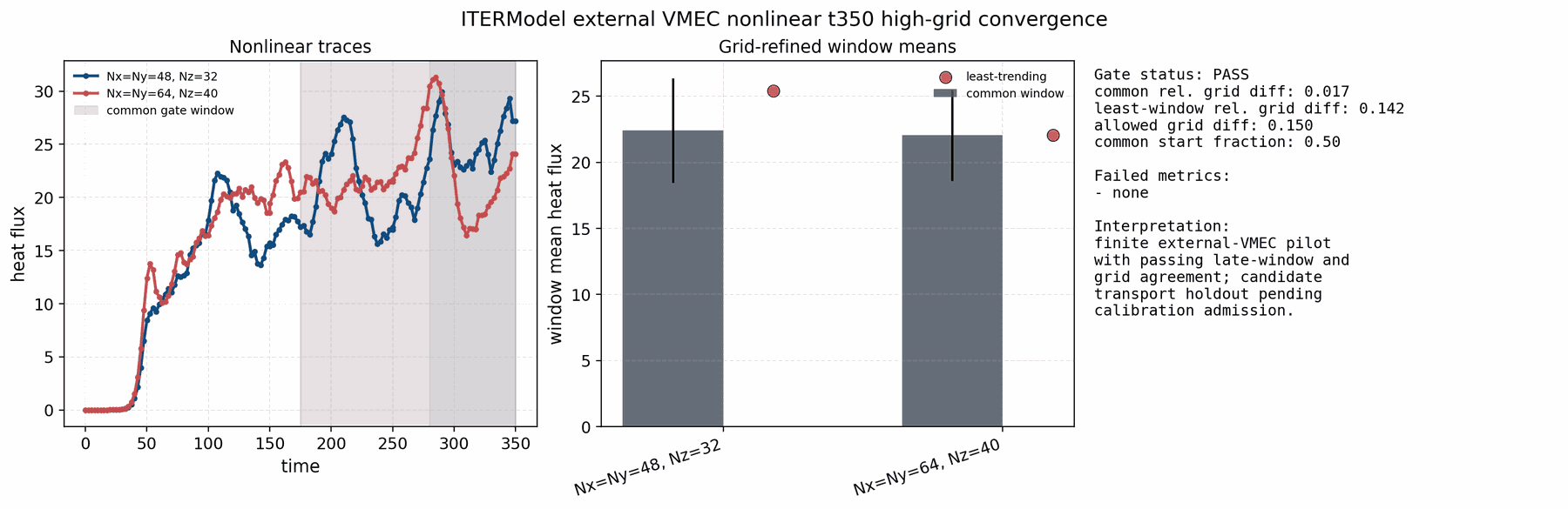
The next screened unstable axisymmetric external-VMEC candidate,
wout_ITERModel_reference.nc, does close the gate after one bounded
extension ladder. The t = 150 pair was already close: the common-window
grid difference was only about 0.073, but the 64x64x40 trace was still
drifting on the common window and the least-window difference was about
0.164, slightly above the 0.15 threshold. Extending the same
48x48x32 and 64x64x40 runs first to t = 250 and then to
t = 350 closes the gate cleanly. At t = 350 the common-window
heat-flux means are about 22.41 and 22.05, the common-window symmetric
relative difference is only 0.0165, the least-window difference is
0.1415, and all trend/CV/sample-count gates pass. ITERModel is therefore
admitted as the second external-VMEC nonlinear transport holdout from this
campaign. As with D-shaped tokamak, this strengthens the negative-transfer
evidence for the current one-constant mixing-length model rather than rescuing
it: the observed heat flux is about 22.0 while the uncalibrated
quasilinear prediction is only about 0.389.
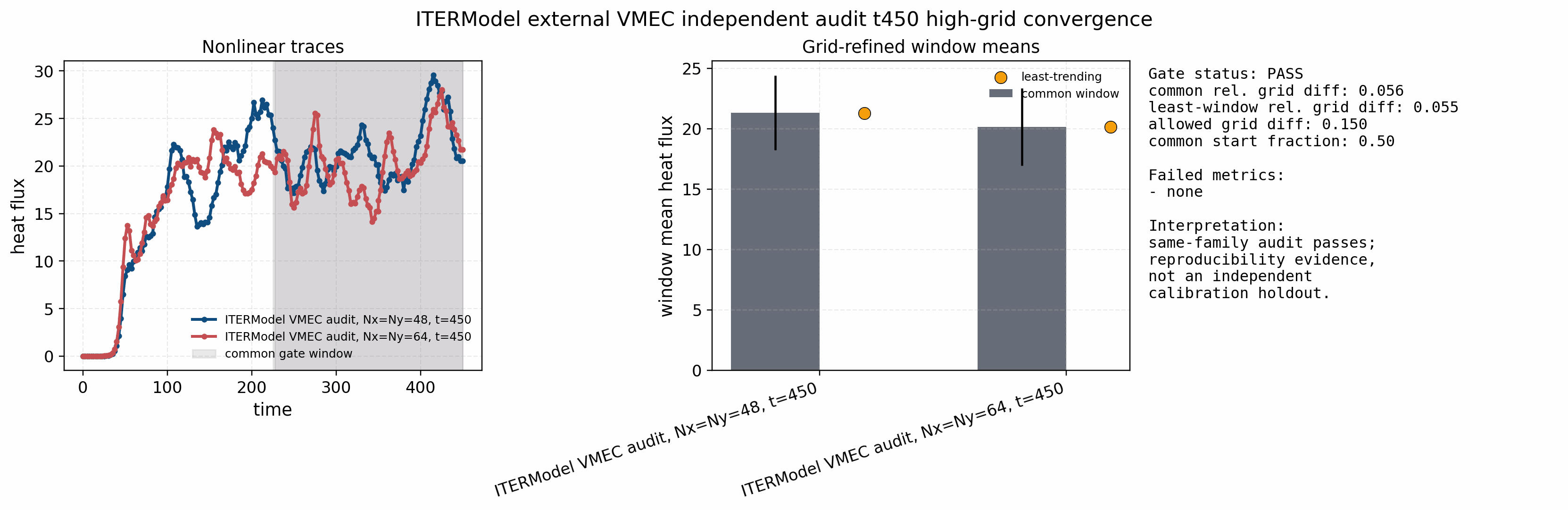
The same ITERModel family was then rerun as an independent t = 450 audit
using the corrected restart ladder. The audit passes the high-grid gate: the
48x48x32 and 64x64x40 common-window heat-flux means are about 21.31
and 20.14, with common-window and least-window symmetric grid differences
0.056 and 0.055. This is useful reproducibility evidence for the
training reference, but it is not admitted as a new quasilinear holdout because
it is not independent of the training-family geometry.
The external-VMEC runbook is now deliberately fail-closed. It requires a
screened linear growth rate of at least gamma = 0.02 before it writes any
nonlinear launch command, and it still requires a matched post-transient
transport window plus passed grid/window convergence before a point can enter
calibration. This blocks three common failure modes: rerunning a same-family
training audit as if it were independent, replaying a family with a recent
failed convergence gate unchanged, and launching expensive nonlinear
simulations from near-marginal linear branches such as the present QI seed.
The current next-holdout screen adds two useful rows to that policy. The
Solovev VMEC equilibrium is now the newest admitted independent nonlinear
holdout (gamma ≈ 0.0944 at ky ≈ 0.2857). Its repaired n48/t250
seed/timestep ensemble passes readiness and the explicit 20% spread gate
with mean heat flux <Q_i> = 1.409 and mean-relative spread 0.1599. The
up-down asymmetric tokamak is also unstable but already represented in the
calibration ledger (gamma ≈ 0.0360 at ky ≈ 0.4762). Solovev is admitted
as negative absolute-QL transfer evidence, not as a promoted predictor.
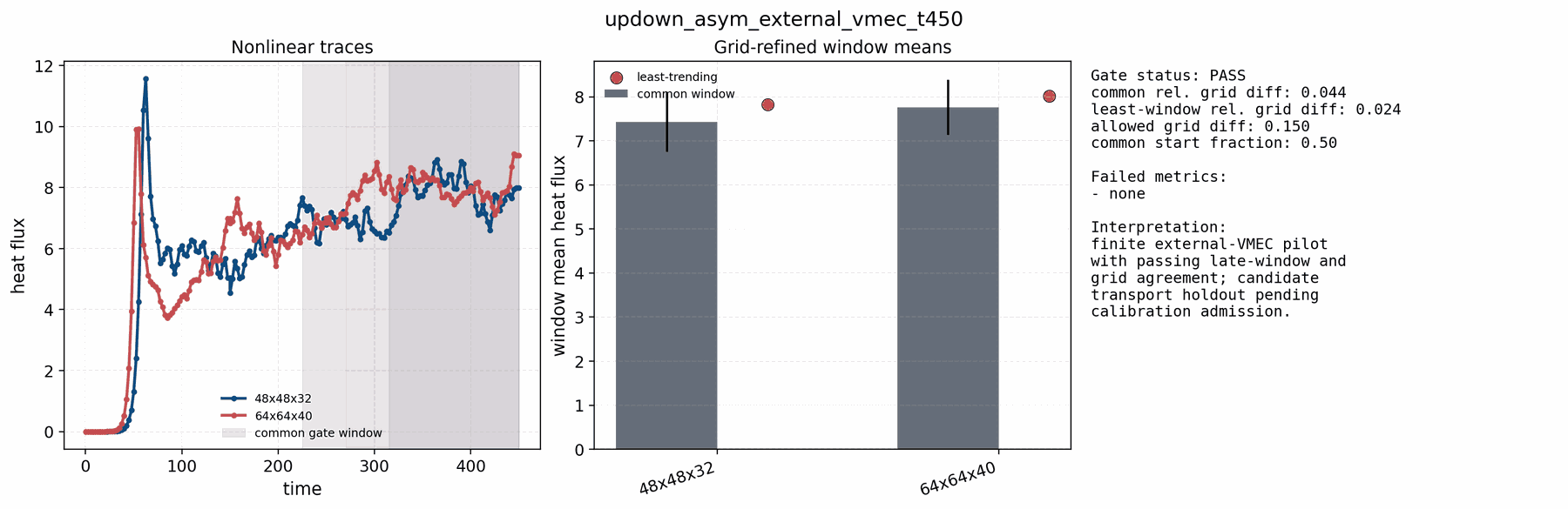
A previously screened unstable external-VMEC tokamak candidate,
wout_up_down_asymmetric_tokamak_reference.nc, also closes after a bounded
extension ladder. At t = 150 the grid difference already passed
(0.138), but the 64x64x40 common-window trend was still too large
(7.32e-3 per time unit). Extending both runs to t = 250 reduced the
common-window relative difference to 0.0411 and the least-window
difference to 0.0499, but the common-window trend on the lower grid was
still slightly above threshold (2.78e-3 versus 2.0e-3). A final
extension to t = 450 closes the gate cleanly: the common-window heat-flux
means are about 7.43 and 7.76, the common-window symmetric relative
difference is 0.0435, the least-window difference is 0.0242, and both
common and least-window trend/CV/sample-count gates pass. This case is now the
third admitted external-VMEC nonlinear transport holdout in the tracked
stellarator/tokamak calibration portfolio.
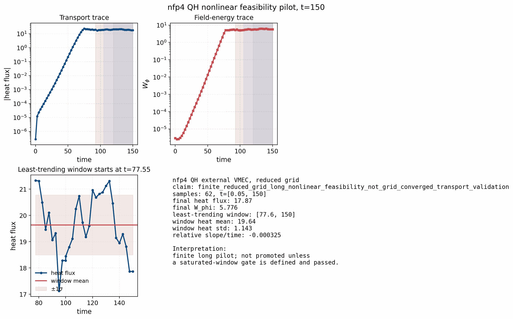
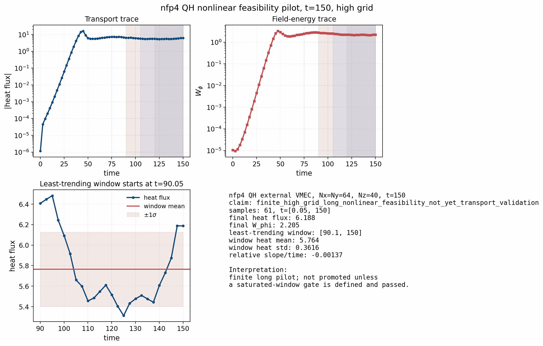
A reduced-grid nonlinear QH pilot has also been run locally at
Nx = Ny = 32, Nz = 24, Nl = 4, Nm = 8, and dt = 0.05 using
the same VMEC fixture. The original t = 20 trace was intentionally not
promoted: its late-half mean heat flux was only about 1.78e-4 and still
growing. The lane has now been extended from the saved nonlinear state to
t = 150. The longer trace reaches a meaningful post-transient heat-flux
level: the least-trending window is t = 77.55 to 150.00, with mean heat
flux about 19.6, standard deviation about 1.14, and relative linear
trend about -3.25e-4 per time unit. This closes the specific concern that
the QH pilot was only measuring a startup/noise-floor heat flux. It is still a
reduced-grid feasibility result, not a calibrated transport holdout, until a
grid/window convergence gate passes.
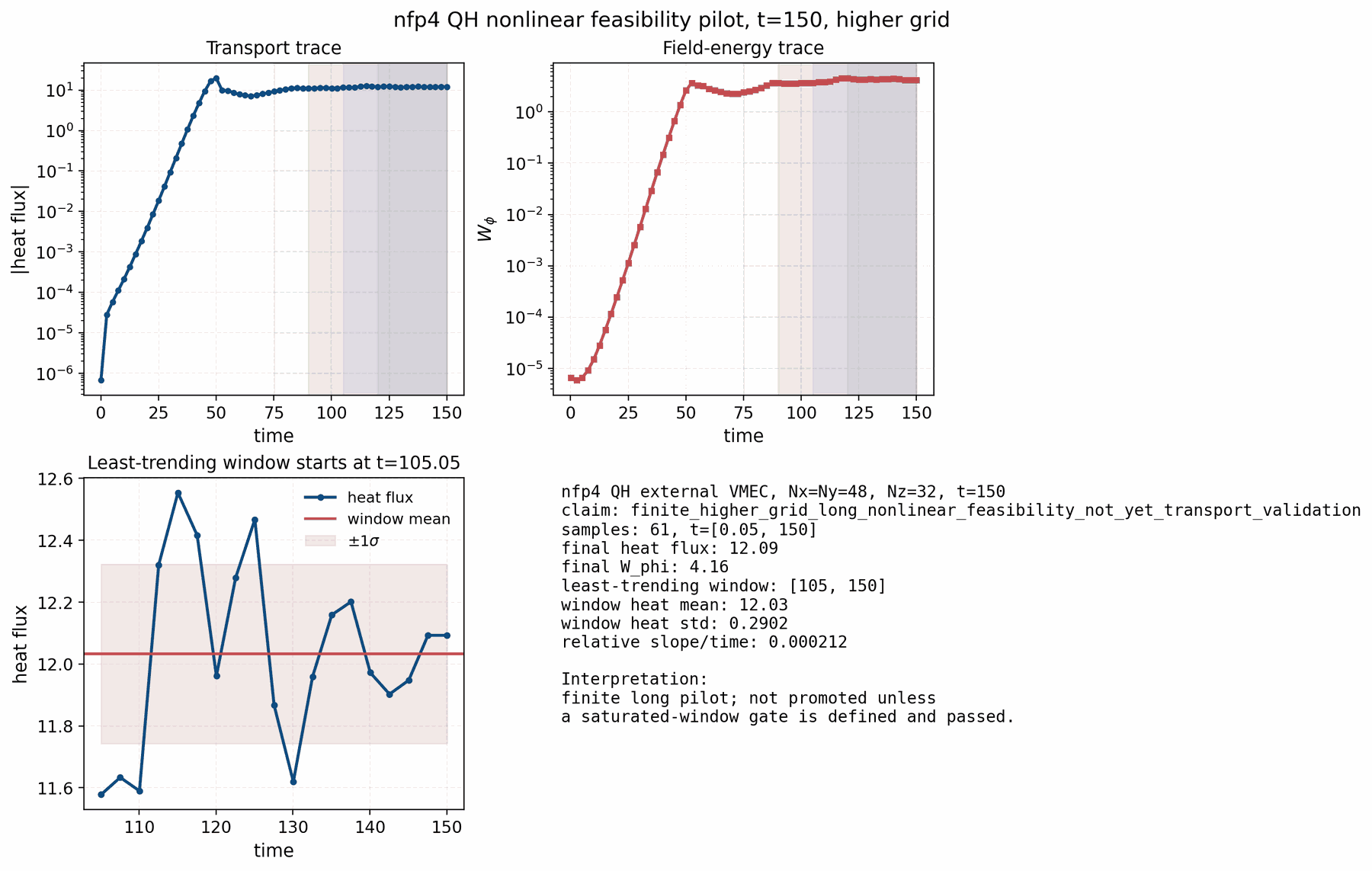
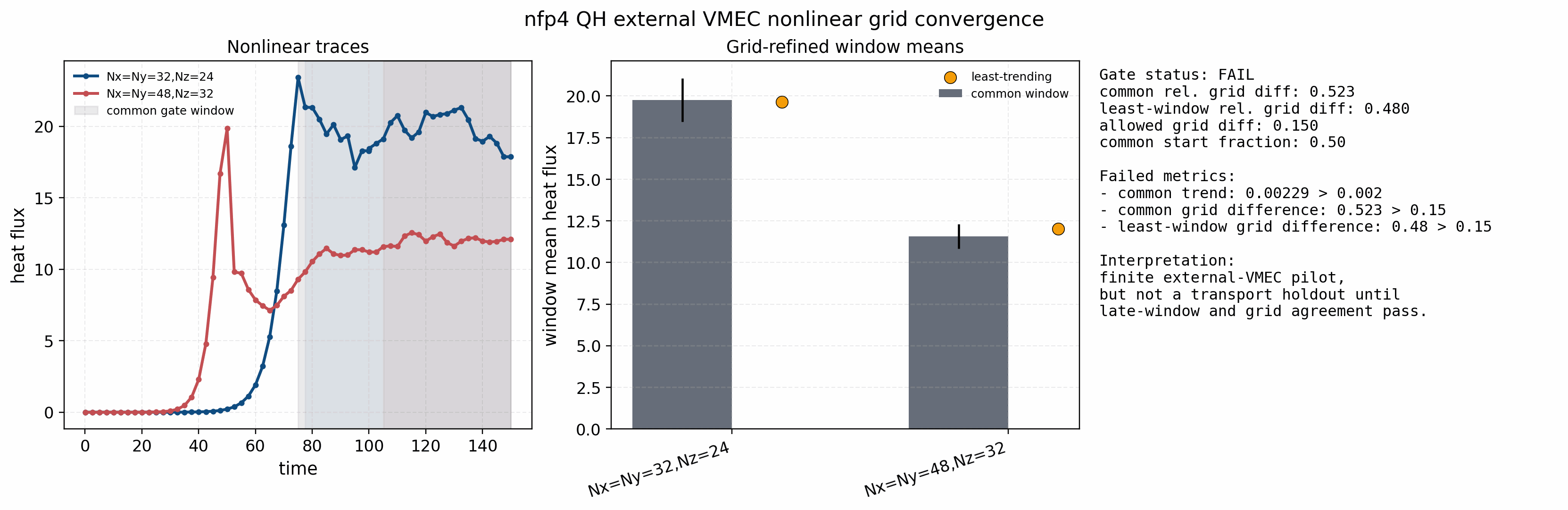
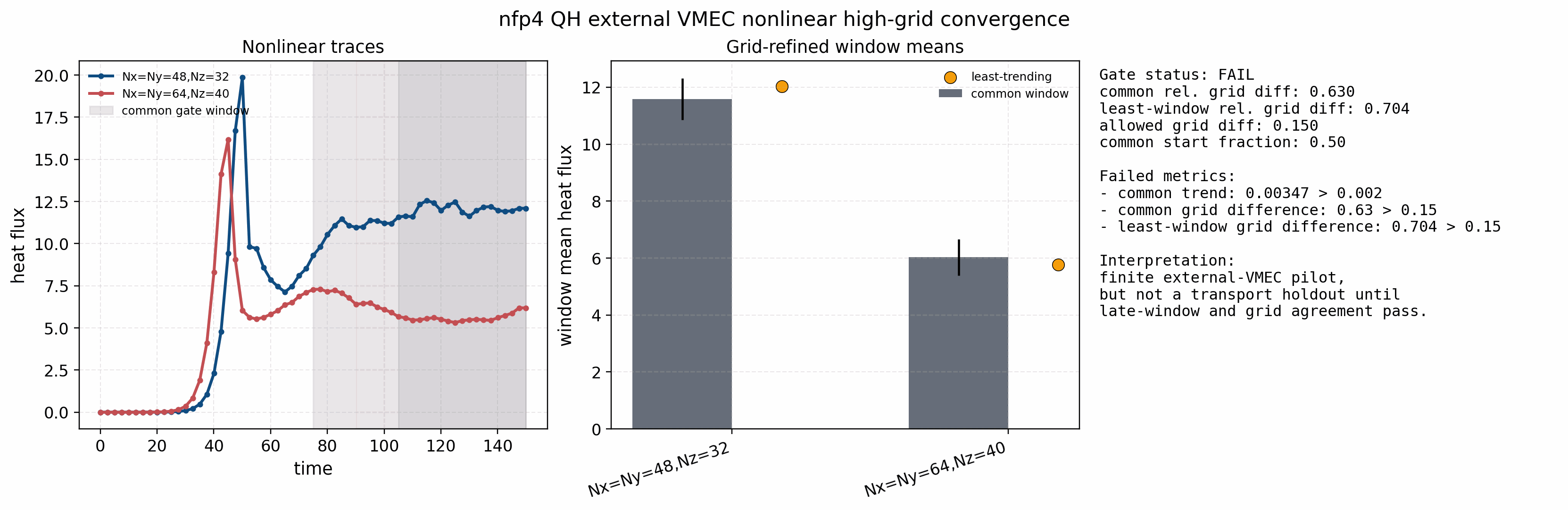
A higher-grid QH companion run at Nx = Ny = 48 and Nz = 32 was then
run on the office GPU to the same t = 150 horizon. It is finite and has a
flat late trace, but the late heat-flux level changes materially: the common
late-window mean is about 11.6 instead of 19.8, and the independently
selected least-trending means are about 12.0 instead of 19.6. The
resulting symmetric relative grid differences are about 0.523 on the
common window and 0.480 on the least-trending windows, both above the
0.15 gate.
The follow-on Nx = Ny = 64 and Nz = 40 run is also finite to
t = 150, but it moves the transport level again instead of confirming the
48x48x32 point: the common-window mean is about 6.0 and the
least-trending mean is about 5.8. The mid-to-high-grid symmetric relative
differences are about 0.630 and 0.704. QH is therefore a useful
negative convergence result, not a new quasilinear calibration holdout.
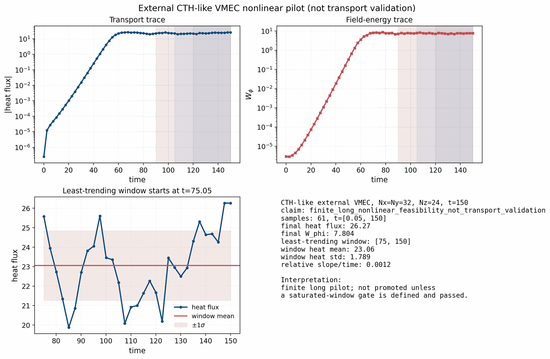
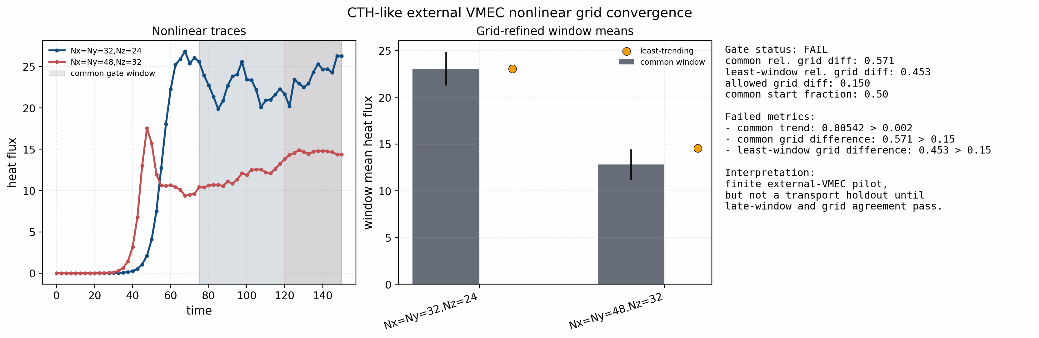
The same reduced-grid protocol was then applied to the CTH-like fixture and
extended on the office GPU to t = 150. The run remains finite and develops a
clear late nonlinear state: the least-trending tracked window is
t = 75.05 to 150.00 with mean heat flux about 23.1, standard
deviation about 1.79, and relative linear trend about 1.2e-3 per time
unit. This is the strongest current external-VMEC nonlinear candidate. It is
still kept as a feasibility pilot, not a transport-calibration holdout, because
no external-VMEC nonlinear acceptance gate has been defined for this fixture
and no independent reference or production-resolution convergence check has
passed yet.
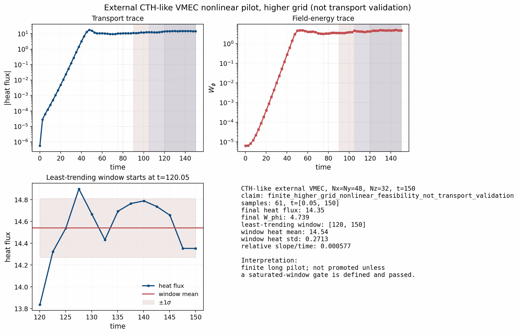
The first bounded grid check repeats the same run at Nx = Ny = 48 and
Nz = 32. It is also finite to t = 150 and has a flatter late trace, but
the transport level changes materially: the common t = 75.05 to 150.00
window has mean heat flux about 12.8 rather than 23.1, and the
least-trending t = 120.05 to 150.00 window has mean heat flux about
14.5. This is a useful negative convergence result. It is retained as
evidence that the original reduced-grid protocol was not sufficient for
calibration.
The explicit convergence gate follows the same evidence chain used in
nonlinear gyrokinetic benchmark papers: time traces and saturated heat-flux
windows are compared, and the candidate is not promoted unless the heat flux is
robust to resolution and window choice. This mirrors the Cyclone and W7-X
time-trace/convergence practice in [Dimits00], [GX], and
[GonzalezJerez22], while the stellarator-domain sensitivity documented by
[Sanchez21] motivates keeping external-VMEC cases behind a conservative gate
until flux-tube and resolution choices are fixed. The first CTH-like pair fails
the common-window stationarity
and grid-refinement requirements: the common-window symmetric relative
heat-flux difference is about 0.571 and the least-trending-window
difference is about 0.453, both above the 0.15 production threshold.
That threshold is intentionally strict enough to match the order of
nonlinear heat-flux convergence tolerances reported for Laguerre-Hermite
gyrokinetic calculations in [GX]. Long turbulent time series need uncertainty
and stopping checks because turbulent flux traces are autocorrelated
[Oberparleiter16], and low-resolution velocity/moment choices can move the
saturated heat flux or even crash [Hoffmann23]. W7-X heat-flux time-series
analyses [Papadopoulos23] are therefore useful context, but the admission
decision still has to be made by explicit gates.
The modified-protocol CTH-like runbook records this distinction explicitly. It
adds the tracked CTH-like linear spectrum point (gamma = 0.0488 at
ky = 0.2857) to the external-VMEC candidate screen and emits a launch
contract only when the failed-family replay is marked as a modified protocol:
n48/n64/n80 grids and t = 150,250,350 horizons after the earlier
32->48 failure. The full modified n48/n64/n80 t=350 sidecar still
fails only the common/least grid-difference metrics: the coarse n48 point
has heat-flux means around 13.4 while the retained n64/n80 means are
around 10.5/9.9. The retained high-grid pair passes at t=250 and
t=350; the late high-grid horizon gate passes with common/least changes
0.018/0.019; and the restart-continued n80 seed/timestep ensemble
passes on t=[350,700] with mean heat flux 9.60, mean-relative spread
0.041, and combined SEM/mean 0.052. The dedicated
tools/release/check_vmec_boozer_gates.py high-grid-admission gate therefore admits
CTH-like as a scoped high-grid holdout while explicitly excluding any full
n48/n64/n80 convergence claim. The shaped-tokamak-pressure repair uses the
same admission policy: full-grid failure is retained as a coarse-grid warning,
while the n64/n80 high-grid, time-horizon, and replicate gates define the
scoped holdout evidence.
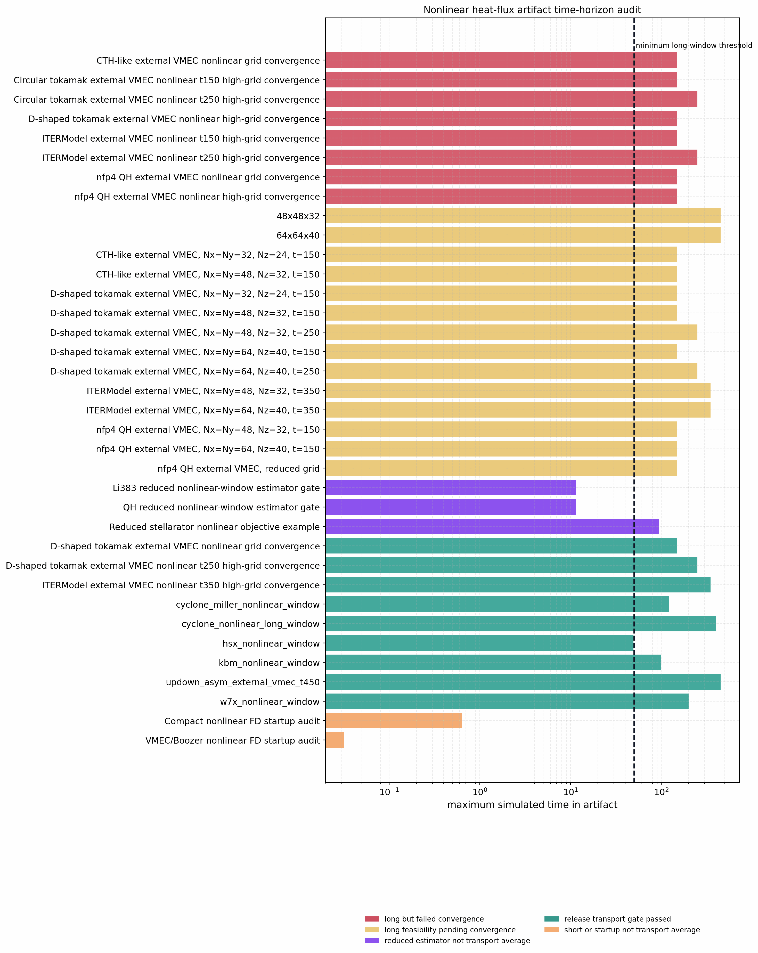
The nonlinear time-horizon audit below is a guardrail for the manuscript and
documentation. It classifies archived heat-flux artifacts by their actual time
coverage and claim level. The long matched nonlinear gates for Cyclone,
Cyclone Miller, KBM, W7-X, and HSX pass the current release comparison
envelopes. D-shaped tokamak passes the external-VMEC t = 250 high-grid
convergence and replicated seed/timestep gates, while circular tokamak passes
the external-VMEC t = 450 high-grid gate and the longer t = 700
replicated seed/timestep gate. CTH-like now enters only through the scoped
high-grid admission policy described above; QH remains a long feasibility
pilot that still needs convergence gates. The compact finite-difference audits
remain startup plumbing checks, and the differentiable nonlinear-window
optimization examples remain reduced-envelope estimators rather than
production nonlinear transport averages.
The normalized W7-X spectrum-shape gate does pass when the linear
heat-flux-weight distribution is compared with the resolved nonlinear
HeatFlux_kyst spectrum from the NetCDF output:
python tools/artifacts/plot_quasilinear_diagnostics.py shape-gate \
  --spectrum docs/_static/quasilinear_w7x_spectrum_scan.quasilinear_spectrum.csv \
  --nonlinear tools_out/final_nonlinear_audit/w7x_gkx_current_adaptive_t200.out.nc \
  --out docs/_static/quasilinear_w7x_spectrum_shape_gate.png \
  --ql-column heat_flux_weight_total \
  --nonlinear-variable Diagnostics/HeatFlux_kyst \
  --tv-gate 0.2 \
  --cosine-gate 0.95 \
  --title "W7-X quasilinear/nonlinear ky-spectrum shape gate"
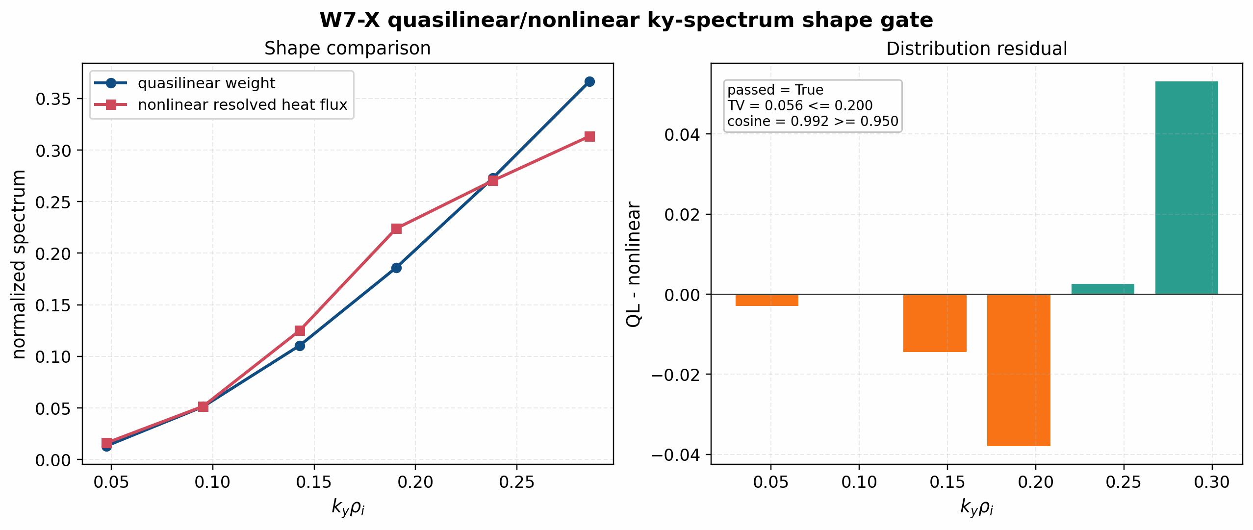
The tracked W7-X shape gate passes with total-variation distance about
0.056 and cosine similarity about 0.992. This supports the
linear-spectrum shape diagnostic for W7-X under the current setup, while the
absolute saturated-flux model remains rejected by the train/holdout report.
The same HSX artifacts also close the first real spectrum-shape gate. This gate
does not use the saturated flux, because the current stable-branch
mixing-length rule would erase the spectrum. Instead it compares the normalized
linear heat-flux-weight spectrum against the normalized nonlinear
HeatFlux_kyst spectrum averaged over the resolved nonlinear diagnostics:
python tools/artifacts/plot_quasilinear_diagnostics.py shape-gate \
  --spectrum docs/_static/quasilinear_hsx_spectrum_scan.quasilinear_spectrum.csv \
  --nonlinear tools_out/final_nonlinear_audit/hsx_nonlinear_t50.out.nc \
  --out docs/_static/quasilinear_hsx_spectrum_shape_gate.png \
  --ql-column heat_flux_weight_total \
  --nonlinear-variable Diagnostics/HeatFlux_kyst \
  --time-max 49.2 \
  --tv-gate 0.2 \
  --cosine-gate 0.95 \
  --title "HSX quasilinear/nonlinear ky-spectrum shape gate"
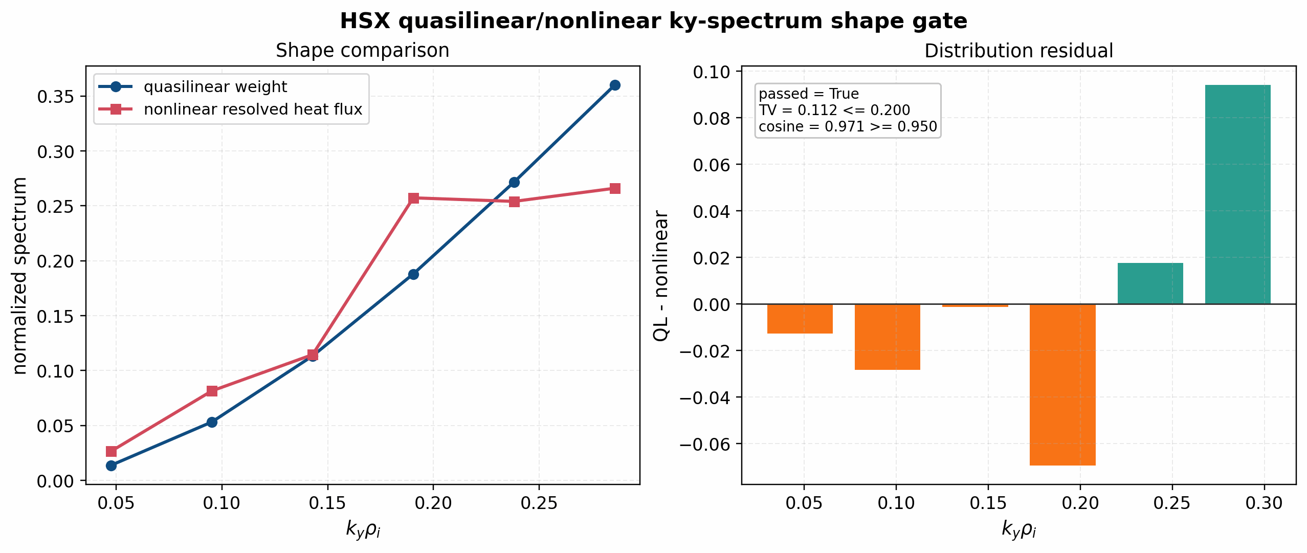
The tracked HSX shape gate passes with total-variation distance about 0.11
and cosine similarity about 0.97. This supports the linear spectrum-shape
diagnostic while still rejecting any absolute saturated-flux claim from the
current uncalibrated rule.
Axisymmetric spectrum-shape gates
The same spectrum-shape extraction is also tracked for the electrostatic
axisymmetric adiabatic-electron nonlinear windows. These gates compare only the
normalized ky distribution of the linear heat-flux weight against the
resolved nonlinear HeatFlux_kyst spectrum. They do not test the absolute
mixing-length heat-flux level.
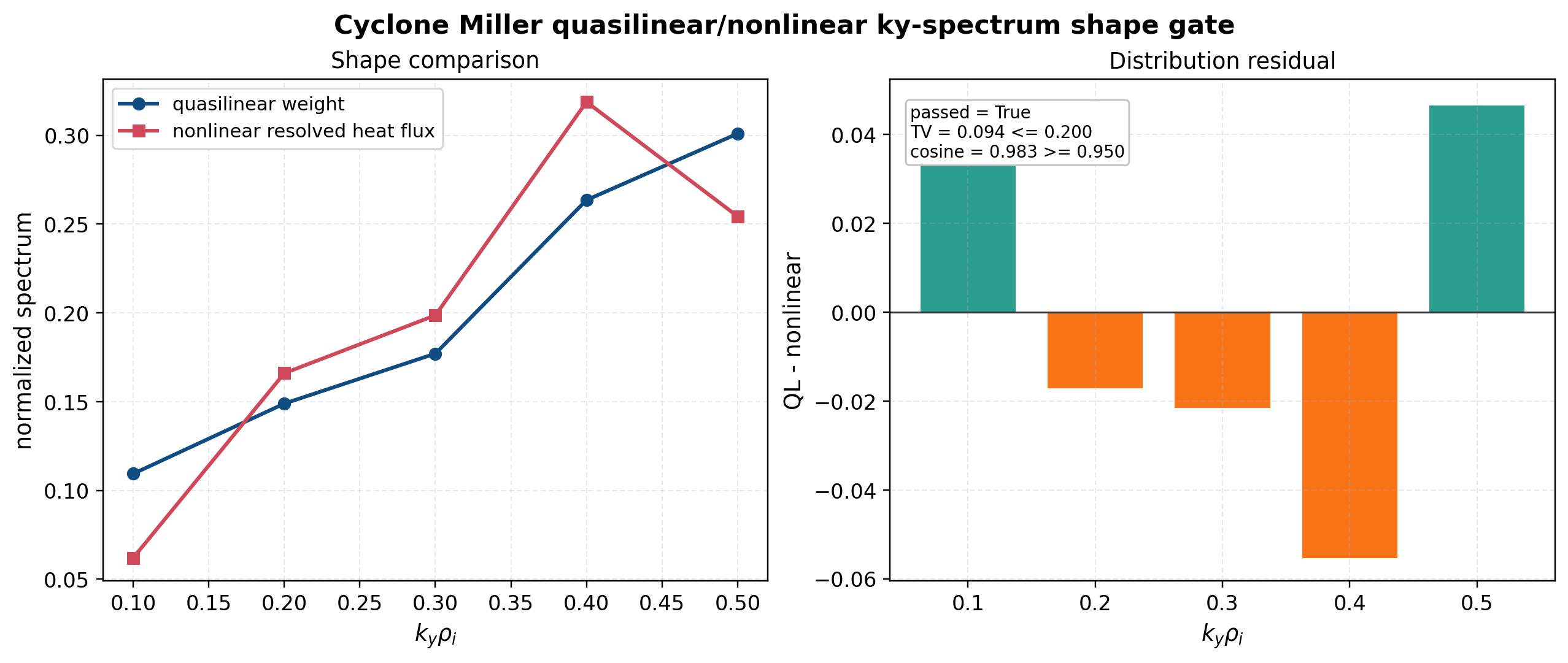
Cyclone Miller passes the initial shape gate with total-variation distance
about 0.094 and cosine similarity about 0.983. This is a useful positive
gate: the linear heat-flux-weight spectrum and the resolved nonlinear heat-flux
spectrum place comparable weight across the scanned ky range under the
current window.
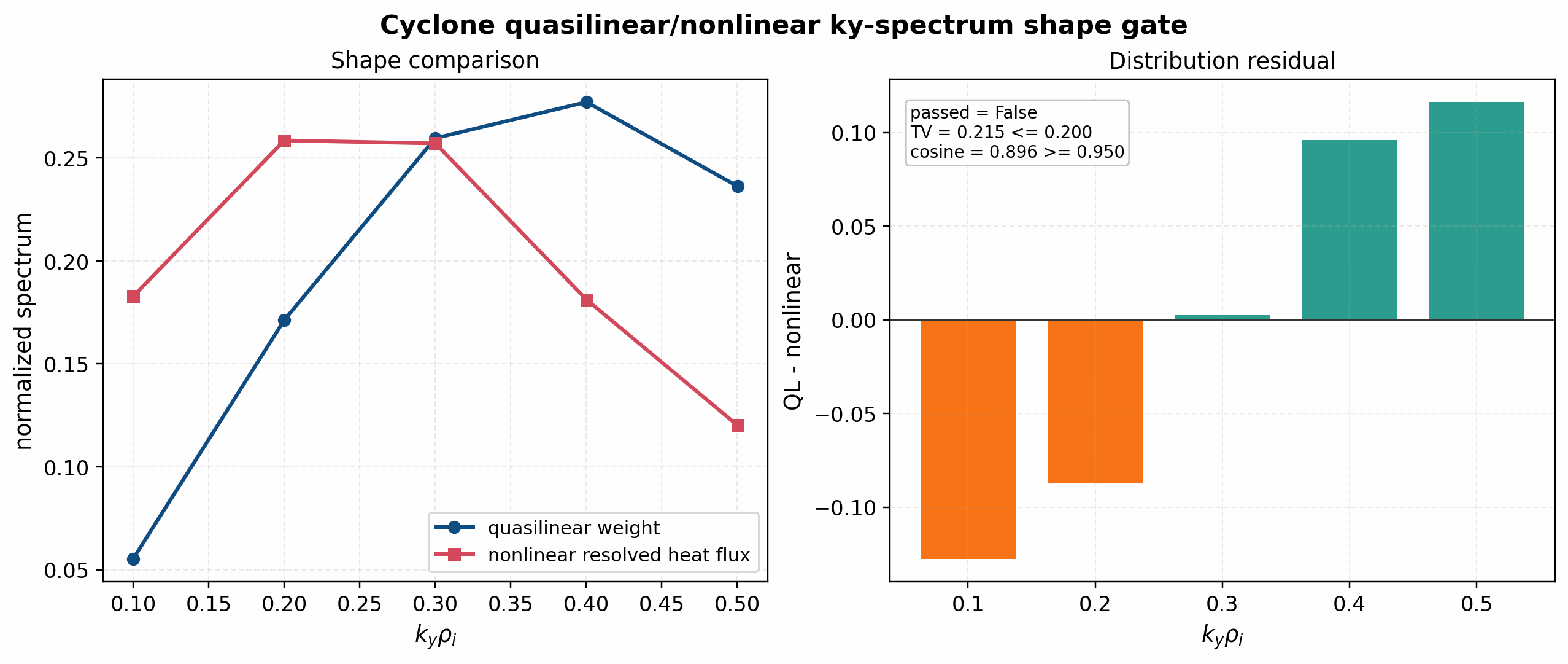
The long-window Cyclone shape gate is intentionally retained as a failed gate:
it gives total-variation distance about 0.215 and cosine similarity about
0.896 against the current TV <= 0.2 and cosine >= 0.95 criteria.
The mismatch is concentrated in the low- and high-ky tails, which points to
a saturation/intensity-model limitation or a window/branch-selection issue
rather than a failed file-ingestion path. This is a paper-facing negative
result and should guide the next quasilinear saturation-model sweep.
KBM is not included in the current spectrum-shape quasilinear gate because the
tracked KBM validation lane is electromagnetic, while the implemented
quasilinear diagnostic currently validates only electrostatic field channels.
KBM should enter this section only after electromagnetic quasilinear weights
for A_parallel and B_parallel have independent normalization and
finite-difference/linear-diagnostic gates.