Operators And Terms
This page documents the implemented operator set in GKX and ties each term to its runtime parameters and source files.
State And Coupled Variable
For each species \(s\), GKX evolves Laguerre-Hermite moments \(G^{(s)}_{\ell m}(k_x,k_y,z,t)\). The field-coupled variable used by the linear operator is
with \(J_\ell^B = J_\ell + J_{\ell-1}\).
In the explicit-time reference-compatible path, streaming is applied to the field-coupled streamed variable built from the same field terms before the Hermite ladder is taken.
Source mapping:
src/gkx/linear.pysrc/gkx/terms/fields.pysrc/gkx/terms/assembly.py
Implemented Linear Operator
The assembled RHS is
Every term has a matching multiplicative weight in TermConfig and
RuntimeTermsConfig.
Gyroaverage And Bessel Factors
The Laguerre gyroaverage coefficients are
Nonlinear electromagnetic terms additionally use \(J_0(\alpha)\) and \(J_1(\alpha)\) on the quadrature grid.
Source mapping:
src/gkx/core/velocity.pysrc/gkx/terms/nonlinear.py
Streaming
The Hermite ladder streaming term is
where \(X\) denotes either \(H\) or the benchmark-compatible streamed variable, depending on the solver path.
Controls:
LinearParams.kpar_scaleRuntimeTermsConfig.streamingboundary/link metadata from the geometry/grid
Mirror
The mirror term uses \(b'(z)\) and couples both Laguerre and Hermite indices:
Curvature And Grad-B
The drift terms are
Controls:
LinearParams.omega_d_scaleRuntimeTermsConfig.curvatureRuntimeTermsConfig.gradb
Diamagnetic Drive
The diamagnetic drive acts through density and temperature-gradient couplings in the low Hermite moments. In code it drives:
m=0through density and perpendicular-energy combinations,m=2through temperature-gradient coupling,m=1andm=3for electromagneticA_parallelterms when enabled.
Controls:
LinearParams.omega_star_scaleLinearParams.R_over_LnLinearParams.R_over_LTiRuntimeTermsConfig.diamagnetic
Collisions
The implemented collisional model is a Lenard-Bernstein-style diagonal damping plus conservation-restoring low-order moment corrections.
Base damping:
where lb_lam is the cached Hermite/Laguerre collision eigenvalue.
The code then reconstructs low moments:
and a temperature-like correction \(\bar{T}\) from m=0 and m=2.
These are added back only into the m=0,1,2 channels.
Claim boundary and extension plan
This is a conserving Lenard–Bernstein/Dougherty-like model, not a complete
linearized gyrokinetic Landau operator. The low-order field-particle correction
is important: the operator cannot be represented only by a diagonal damping
array. The implementation contract for collision extensions therefore has two
paths. Both receive a post-field CollisionContext so finite-Larmor-radius
models can distinguish the evolved distribution \(G\) from the
Hamiltonian response \(H\):
apply(context)for the complete unit-weight RHS, including low-rank or dense field-particle terms;SplitCollisionOperator.split_step(context, dt)as an optional contract only when the model supplies a mathematically valid exact or implicit finite-time update. The runtime does not automatically route this method yet. Diagonal hypercollision splitting must not be reused for a non-diagonal conserving operator.
The first path is available from Python through
nonlinear_rhs_cached(..., collision_operator=operator). The callback must
return a JAX array with the state shape. GKX removes the built-in
collision contribution before adding terms.collisions * operator.apply(...);
hypercollisions remain independent:
class CollisionModel:
    def apply(self, context):
        return collision_rhs(
            context.distribution,
            context.hamiltonian,
            context.cache,
            context.parameters,
        )

rhs, fields = nonlinear_rhs_cached(
    state, cache, parameters, terms,
    collision_operator=CollisionModel(),
)
The callback is evaluated after the field solve and traced by JAX, so its array
operations remain differentiable. context.fields carries phi, apar,
and bpar; context.hamiltonian uses the same enabled-field policy as the
gyrokinetic RHS. This avoids silently replacing a finite-\(b\)
field-particle model by a \(G\)-only approximation.
This contract is also used by the generated equal-species finite-wavelength
Coulomb and Sugama validation operators described below. Those operators are
research validation paths, not input-file options: TOML selection and split
integration remain disabled until the full zonal-response acceptance gate
passes.
The built-in collision_split policy consequently splits only diagonal
hypercollisions. The conserving collision term remains in the Runge–Kutta or
IMEX RHS, including its field-particle corrections. Earlier implementations
removed the complete collision RHS and advanced only its diagonal part; that
violated the stated conservation model and is no longer supported.
collision_invariant_rates returns the discrete long-wavelength density,
parallel-momentum, and thermal-energy rates of a state-shaped contribution.
collision_quadratic_rate evaluates
\(\operatorname{Re}\langle H,C[H]\rangle\) with optional species/spatial
weights. Release tests use these functions to verify a local-Maxwellian null
space, all three fluid invariants, and dissipative non-fluid response at
\(b=0\).
multispecies_collision_invariant_rates supplies the stricter acceptance
contract for a species-coupled model. For species-normalized coefficients it
returns each particle-density rate and the physically weighted sums
The model is promotable only when every particle rate and both summed rates vanish to discretization tolerance. This diagnostic is implemented and autodiff-tested; it does not by itself promote a multispecies collision model.
Reduced drift-kinetic Sugama equation gate
drift_kinetic_sugama_six_moment_contribution and
drift_kinetic_coulomb_six_moment_contribution implement the complete
like-species six-gyromoment matrices reported in Appendix C, equations
(C6a)–(C6f) and (C9a)–(C9f), of the improved Sugama moment formulation. In GKX ordering, the nontrivial
moment vector is
where the signs on Laguerre moments account for the code’s polynomial convention. The operator is \(\nu_s M\boldsymbol{N}\) with two symmetric blocks. The thermal block is
and the heat-flux block is
For the exact linearized Coulomb operator, the corresponding blocks are
Tests evaluate every matrix entry, symmetry, non-positive eigenvalues, the Maxwellian thermal null direction, density/momentum/energy invariants, and a collision-frequency JVP against centered finite differences. This is a real high-collisionality reduced operator and an equation-level acceptance gate for the future coefficient generator. It intentionally returns zero outside the six-moment projection and is therefore not selected by TOML or presented as a full Hermite–Laguerre hierarchy, finite-Larmor-radius, multispecies, or production Sugama/Coulomb implementation.
The same C6/C9 coefficients also exercise the production table boundary. The maintainer command
python tools/artifacts/build_linear_validation_artifacts.py collision-table
evaluates the analytic coefficients with 80-decimal-digit mpmath
arithmetic, writes a deterministic float64 array, and records its SHA-256,
mode ordering, polynomial convention, source equations, and claim scope in a
JSON sidecar. load_collision_moment_matrix(model) verifies the package-data
checksum before returning a host array. apply_collision_moment_matrix then
packs (ell,m) into the paper’s Hermite-major ordering, applies either one
shared or one matrix per species in JAX, and restores the state layout.
interpolate_collision_moment_matrix provides the finite-\(b\) runtime
boundary: it linearly interpolates a strictly increasing \(k_\perp\) table
on device, clamps only outside the generated range, and accepts either one
shared table, an explicit table per species, or an ordered target/source pair
table with shape (target, source, kperp, moment, moment). Pair tables use
the target species’ \(k_\perp\) field, matching the species-dependent
gyroradius convention, and return the spatial matrix layout consumed directly
by apply_multispecies_collision_moment_matrix. The resulting matrix may
vary at every perpendicular/parallel grid point without leaving traced JAX
execution.
TabulatedMultispeciesCollisionOperator exposes this finite-wavelength
boundary through the standard collision protocol. It is a JAX pytree containing the coefficient
grid and fully assembled, collision-frequency-weighted pair table; its
apply method obtains \(k_\perp\rho_s=\sqrt{b_s}\) from the solver cache,
interpolates each target/source block, and acts on the post-field Hamiltonian.
In contrast, DriftKineticMomentCollisionOperator implements the
drift-kinetic convention of Frei, Ernst & Ricci (2022), Eq. (73): its dense
matrix acts directly on evolved gyrocenter moments because \(f\simeq g\)
in that limit. A full-RHS gate checks both conventions independently.
Generated tables, rather than the runtime
operator, own directed-frequency normalization and coefficient provenance.
Tests require node and endpoint identity, generated-table/direct-equation
identity for both models, species-local spatial application, and JVP/finite-
difference agreement through state amplitude, collision frequency, and an
interior \(k_\perp\) target. The ordered-pair gate additionally checks JIT
application, pair-block identity, zero-\(b\) multispecies invariants, and
target-species-leading spatial interpolation. A separate held-out gate constructs matrices
from the implemented Mandell–Dorland–Landreman finite-Larmor-radius collision
equations, never from the interpolator, and recovers the expected second-order
table-spacing convergence against direct operator evaluations.
This table boundary now supports two deliberately distinct levels. The small package-data table contains only the drift-kinetic six-moment matrices and is used for fast equation and API tests; repeating it at higher resolution would not create finite-\(b\) physics. The offline generator separately builds the complete equal-species diagonal Coulomb test/field matrices and polarization vectors at arbitrary retained Hermite–Laguerre order. Original- and improved-Sugama field matrices are derived from that exact Coulomb test table. These larger archives stay outside the package and are accepted only through the slab-ITG and collisional-zonal runtime gates.
The first exact primitive used by that generated hierarchy is
bessel_laguerre_kernels(bessel_argument, n_max) in core.velocity. It
implements Frei et al. (2021), equation (2.13),
where \(B=k_\perp v_{\mathrm{th}}/\Omega\), using the stable recurrence \(K_{n+1}=K_n B^2/[4(n+1)]\). These coefficients expand \(J_0(B\sqrt{x})\) in Laguerre polynomials and decay factorially, motivating the paper’s finite-sum rule \(N>B^2/4\). The validation suite compares them with an independent 96-point Gauss–Laguerre projection, verifies the reported sub-0.1% tail at \(B=1,N=3\), and checks JIT and JVP/finite-difference agreement. This validates one generator building block; it does not supply the collision-specific coupling coefficients.
associated_bessel_laguerre_coefficients implements the complete
equation-(2.12) prefactor for arbitrary non-negative Bessel order \(m\),
Direct reconstructions of \(J_m(b\sqrt{x})\) for \(m=0,1,2\) agree with an independent special-function implementation over the tested wavenumber and velocity domain. This closes the Bessel-expansion layer used by the collision sums, but not the speed-function or test-/field-particle contractions themselves.
The offline generator also evaluates the Coulomb speed integrals
\(e_{ab}^k\) and \(E_{ab}^k\) from Appendix A, equations (A8a)–(A8b),
with 80-digit arithmetic. Orders zero through five at three unequal thermal-
speed ratios agree with direct improper quadrature of their defining
integrals. coulomb_speed_moments now composes those integrals into the
velocity-integrated test and field functions in equations (A5) and (A13).
Six cases spanning \(0.25\leq m_a/m_b\leq4\),
\(0.5\leq T_a/T_b\leq3\), and spherical order zero through three agree
with direct three-dimensional Maxwellian quadrature of equations (A2) and
(A10). The equal-species density moment vanishes and the momentum test/field
pieces cancel. These remain generator internals because the complete matrix
contractions that consume them are not yet implemented.
The same generator evaluates equation (3.10)’s monomial coefficients for \(L_j^{p+1/2}(x)\). Independent generalized-Laguerre evaluations verify tensor orders \(p=0,1,4\) through polynomial order \(j=8\). The next basis-transform coefficients are cancellation-sensitive. Their provenance is now closed: the base transform is Appendix A, equation (A4), of Jorge, Ricci & Loureiro (2017), and the finite-\(m\) transform and inverse are Appendix B, equations (B5)–(B6), of Jorge, Frei & Ricci (2019). Both formulas were audited against their defining basis identity rather than accepted as printed.
The isotropic base transform and inverse are now implemented in the offline
generator from equations (A4) and (A3), respectively. Selected coefficients
agree with independent 80-point Gauss–Hermite/Gauss–Laguerre velocity
projections, including the hand identities \(cP_1=H_1/2\) and
\(c^2P_2=H_2/4+L_1/2\). Forward/inverse products close through total degree
12 with maximum error 8.73e-15 even though that shell’s condition number is
1.93e8. All nested sums remain multiprecision until the final table cast.
The finite-\(m\) forward transform is now generated as a complete lower- triangular parity block. Under SciPy’s associated-Legendre convention, a literal equation-(B5) transcription gives half the independently projected \(m=0\) coefficients and the opposite sign for odd \(m\); the required factor \(2(-1)^m\) is fixed independently by the \(m=0\) endpoint, eight velocity-space projections, and pointwise reconstruction. Unlike the isotropic map, every lower reduced-degree shell of the same parity is retained. Even and odd blocks through reduced degree six reconstruct the physical basis for \(m=0,1,2,3\). Literal equation (B6) fails the finite-\(m\) inverse identity. Equation (3.33) of Frei et al. (2021), which includes the weighted Laguerre-product contraction omitted from that direct normalization, matches every entry of independently inverted degree-six blocks for \(m=0,1,2,3\). Complete 80-digit block inversion remains the independent oracle; equation (3.33) supplies the scalar inverse used by collision-matrix assembly. This closes coefficient generation, not the test-/field-particle contractions or their transport validation.
The next algebraic layer is also generated and independently checked.
laguerre_product_expansion_coefficient implements both the unweighted
product in equations (3.44)–(3.45) and the \(x^m\)-weighted product in
equations (3.36)–(3.37) of Frei et al. (2021). Pointwise polynomial
reconstruction covers \(m=0,1,2\). Combining that product with the
finite-\(m\) transform and \(K_n(b)\) yields
gyroaveraged_spherical_moment_coefficient, one coefficient of equation
(3.35). Six coefficients through \(m=3\) and \(b=1.3\) agree with
independent Bessel-weighted velocity projection; 20- and 32-term Bessel sums
also agree. This validates the gyro-moment-to-spherical-moment map consumed by
the Coulomb contractions.
The offline generator now contracts equations (3.48)–(3.49) into complete
finite-\(b\) test- and field-particle matrices with explicit Hermite,
Laguerre, spherical-harmonic, and Bessel truncations. Unlike-species generation
keeps \(b_a=k_\perp\rho_a\) in the test and outer gyroaverage factors and
\(b_b=k_\perp\rho_b\) in the field-particle source moments; a regression
holds \(b_a\) fixed and verifies that only the field block changes with
\(b_b\). At \(b=0\), every
published nonzero six-moment Coulomb entry is recovered. The larger generated
block is symmetric to 8.33e-17, negative semidefinite, and preserves
density, parallel momentum, and thermal energy within 3.3e-16. Equation
(3.41)’s \(\Pi^{pjm}\) agrees with five independent
\(J_0J_m\)-weighted velocity projections to about \(10^{-13}\).
Equation (3.50) remains four separate vectors multiplying
\(q_a\phi/T_a\) and \(q_b\phi/T_b\), because quasineutrality couples
species; like-species test/field polarization cancels. This closes the offline
algebra, not runtime multispecies assembly or transport promotion.
The reproducible algebra/convergence artifact is generated with
python tools/artifacts/build_linear_validation_artifacts.py collision-verification
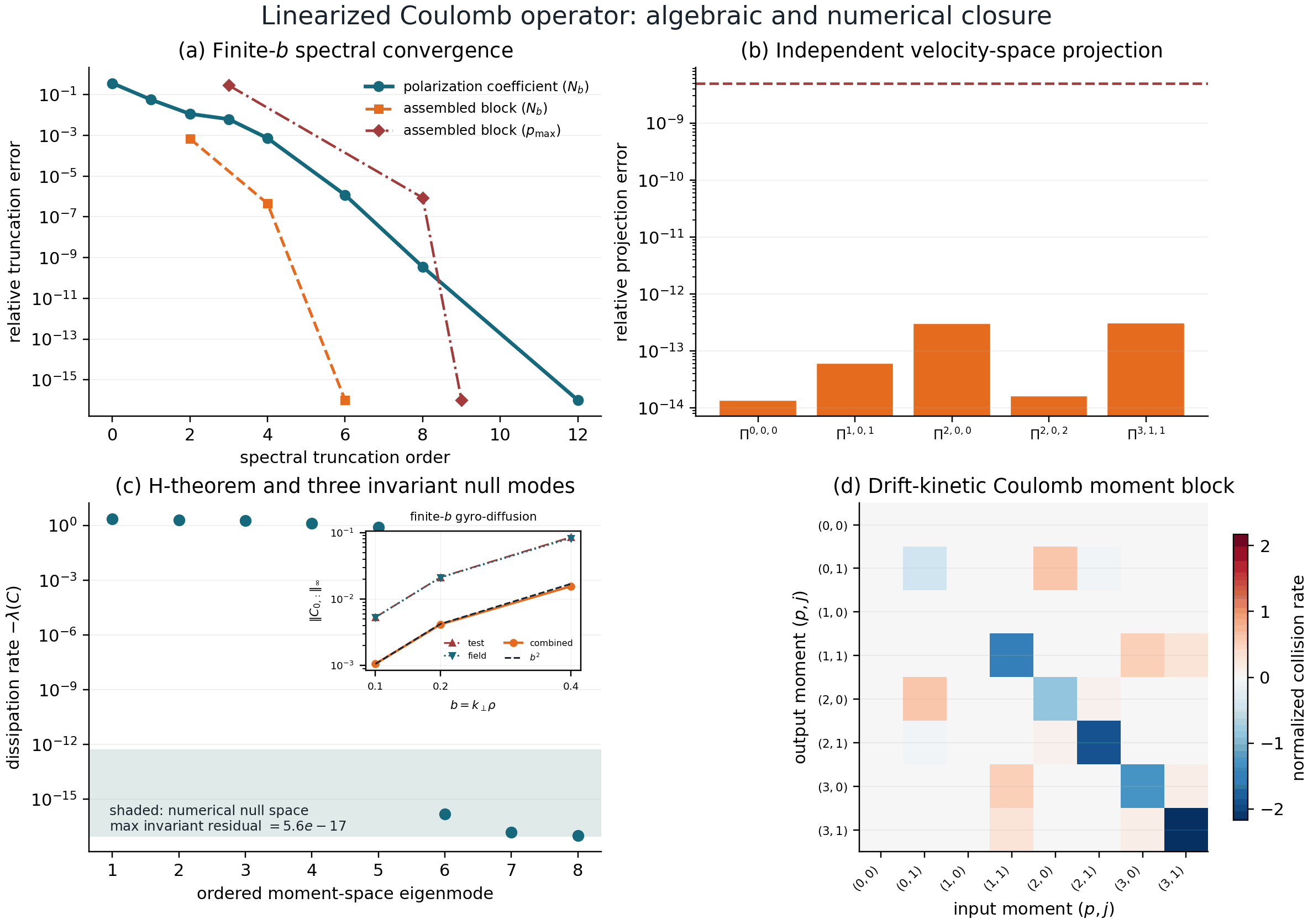
Offline Coulomb-operator closure. Panel (a) shows Bessel–Laguerre
convergence of a finite-\(b\) polarization coefficient to a 24-term
reference, Bessel convergence of an assembled 4-by-4 collision block, and
the independent spherical/radial hierarchy convergence of that block;
panel (b) compares five generated coefficients with independent
80-by-80 Gauss–Hermite/Laguerre velocity projection; panel (c) shows five
dissipative modes and the three density, parallel-momentum, and thermal-
energy null modes, while its inset verifies leading \(O(b^2)\) classical
gyro-diffusion away from the drift-kinetic limit; panel (d) exposes the
complete retained drift-kinetic moment block. The machine-readable gate is
stored beside the figure in collision_operator_verification.json.
The largest direct-projection relative error is \(3.2\times10^{-13}\); the published-coefficient, symmetry, and invariant residuals are at or below \(1.2\times10^{-16}\). At \(b=0.8\), the assembled 4-by-4 block changes by \(4.50\times10^{-7}\) between Bessel orders four and six at the admitted \((p_{\max},j_{\max})=(8,4)\) spherical cutoff. The former default spherical cutoff \((p_{\max},j_{\max})=(3,1)\) is rejected because it differs by 29% from the converged \((9,4)\) reference. The admitted \((8,4)\) block reduces that error to \(8.68\times10^{-7}\). These checks implement the conservation, Maxwellian-null, adjointness, and H-theorem requirements emphasized by Abel et al. (2008) and the finite-\(b\) moment algebra of Frei et al. (2021). The quadrature check is a deterministic manufactured-projection test: it verifies the generated operator against its continuous velocity-space definition, independently of the symbolic contraction path.
Physical promotion is deliberately stricter. After multispecies quasineutrality is assembled, the operator must reproduce Spitzer–Härm/ Braginskii transport, the weakly collisional Hermite–Laguerre convergence and finite-\(b\) ITG scans, and the separately defined collisionless Rosenbluth–Hinton residual and Hinton–Rosenbluth collisional damping traces. The target resolutions, observables, and figure protocols follow Figures 4–9 of Frei et al. (2021) and the conductivity study of Frei, Ernst & Ricci (2022). Until those runtime gates pass, the panel supports operator algebra and numerical closure, not a production Landau-transport claim.
The runtime research boundary now mirrors the same decomposition.
FiniteWavelengthCoulombOperator stores test, field, and four polarization
tables with independent target/source Bessel-argument axes
\(B_a=k_\perp v_{Ta}/\Omega_a\). The gyrokinetic cache stores
\(b_a=k_\perp^2T_am_a/(q_aB)^2\), so a bilinear JAX interpolator evaluates
the table at \(B_a=\sqrt{2b_a}\) and \(B_b=\sqrt{2b_b}\); the resolved
kernel applies equations (3.48)–(3.49) to gyrocenter moments \(G_a\) and
\(G_b\), then adds equation (3.50) using the solved potential and distinct
\(q_a/T_a\) and \(q_b/T_b\) factors. It intentionally does not apply
the matrices to build_H because that would double-count the pullback
polarization.
For a single like-species plasma,
EqualSpeciesFiniteWavelengthCoulombOperator stores only the physical
diagonal \(B_a=B_b\) of those tables. This is not a reduced collision
model: it retains the same test, field, and four polarization terms, while
avoiding coefficient generation on target/source wavelength pairs that cannot
occur in the one-ion-species problem. Its one-dimensional interpolation is
JIT compatible and differentiable with respect to the local Bessel argument.
Multispecies input is rejected rather than silently applying the diagonal
assumption.
Independent Python pair loops, JIT execution, JVP/finite-difference checks, like-species polarization cancellation, generated-coefficient application, full-pair/diagonal identity, and the complete cached linear-RHS seam pass. This closes runtime algebra and differentiable interpolation. It does not yet close Hermite/Laguerre truncation or any transport benchmark; therefore this class remains a Python research API and has no input-file selector.
Finite-\(b\) conservation must be stated carefully. Collisions are local at the particle position, whereas the evolved moments are defined at the gyrocenter. Consequently, the gyrocenter density row is not a null row at finite \(k_\perp\rho\); it represents classical gyro-diffusion. The tracked verification artifact recovers the density null at \(b=0\), obtains a nonzero finite-\(b\) row, and measures the expected leading \(O(b^2)\) scaling separately for the test, field, and combined rows. Equation (3.35) maps a gyrocenter distribution to particle moments; it is not an inverse of the gyrophase average in equation (3.5). Local particle-space conservation therefore cannot be inferred by applying that moment map to the already gyroaveraged collision matrix. A future direct particle-coordinate implementation must test equations (3.2)–(3.4) before gyroaveraging instead.
The multiprecision generator uses exact integer combinatorics for polynomial binomial factors, memoizes repeated inverse-basis contractions within one assembly, and retains arbitrary precision where gamma functions and non-integer coefficients require it. These changes preserve the generated blocks bit for bit while reducing a representative assembly from 34.1 to 3.46 seconds. Applying equation (3.35)’s \(M^{000}\) map to the gyroaveraged collision matrix leaves a nonzero residual, as equation (3.5) predicts; that quantity is retained only as a rejected diagnostic, not a conservation or resolution gate.
The lowest-order multispecies drift-kinetic boundary is also implemented
without assuming equal species. For an ordered pair \((a,b)\),
drift_kinetic_sugama_pair_matrices evaluates Appendix C, equations
(C4)–(C5), of Frei, Ernst & Ricci (2022) as
Here \(T_{ab}\) and \(F_{ab}\) are the published test- and
field-particle matrices on the eight-mode Nl=2, Nm=4 space; coefficients
outside the six active moments are exactly zero. The helper returns matrices
normalized by the directed frequency
so callers retain explicit ownership of normalization. The separate
apply_multispecies_collision_moment_matrix contract stores target species
first and source species second, applies all source blocks in one JAX
contraction, and supports pointwise spatial matrices. At equal mass and
temperature, \(T_{aa}+F_{aa}\) reproduces the independent 80-digit C6
table. assemble_drift_kinetic_sugama_matrix vectorizes all ordered pairs
and adds each test-particle block to its target-species diagonal. An unequal
ion-pair gate checks published coefficients directly; a physical
directed-frequency gate conserves each species’ particles and total momentum
and thermal energy, produces a negative weighted quadratic rate, and matches
finite differences through \(\sigma\) and \(\tau\). An independent
matrix-exponential trajectory preserves those invariants through unequal-
species relaxation and reduces the collision residual by more than five
orders of magnitude.
For Python solver experiments,
DriftKineticMomentCollisionOperator.from_species wraps that matrix in the
standard collision protocol. Its apply method uses
CollisionContext.distribution as required by the drift-kinetic limit. A
collision-only two-species linear-RHS gate verifies a
nonzero response and the same physical invariants. The operator is a JAX
pytree, preserving differentiation when species parameters are constructed
inside an objective.
This is the original Sugama model’s real low-order drift-kinetic projection. It is useful for reduced-model verification but is not an arbitrary-moment hierarchy or a finite-\(b\) multispecies runtime model.
Lowest-order improved-Sugama correction
drift_kinetic_improved_sugama_pair_matrices adds the complete low-order
test- and field-particle corrections in Appendix C, equations (101)–(102), to
the original-Sugama ordered pair. The paper labels the driven moment with a
superscript and the response with a subscript, so the published coefficient
array is transposed once into the runtime row/column application convention.
For equal species the test correction vanishes and the field correction
reproduces equations (103a)–(103c) from an independently generated 80-digit
table. Unequal-mass and unequal-temperature pair coefficients are checked
directly, and their assembled matrix conserves particle number, total parallel
momentum, and total thermal energy. At equal species the correction reduces
the heat-flow-block Frobenius distance to the Coulomb matrix from about
0.521 to 0.205; the equal-temperature multispecies weighted symmetric
operator is non-positive over the complete reduced moment space.
assemble_drift_kinetic_improved_sugama_matrix and
DriftKineticMomentCollisionOperator.from_improved_species expose this equation slice
through the same vectorized JAX and collision-protocol paths. This is a
friction-flow matrix validation, not a parallel-conductivity claim. The
published conductivity comparison retains more moments and reports that the
original operator can underpredict current by at least 10%, while the improved
operator approaches Coulomb within 1%; GKX therefore keeps
conductivity promotion blocked until the arbitrary-moment correction hierarchy
and its driven steady-state gate are implemented.
Driven parallel-current response
The response algorithm needed by that promotion is now an explicit JAX contract. For a Maxwellian electron background, equation (81) of Frei, Ernst & Ricci (2022) linearizes to
where \(\widehat E=eE/(v_{Te}m_e)\) and the electron current follows from
\(u_e=N_e^{10}v_{Te}/\sqrt{2}\). parallel_electric_field_source
constructs this source in Hermite-major ordering, and
solve_driven_collision_response solves
\(C N_e+s_E=0\) after explicitly removing invariant or intentionally
truncated modes. The solve uses jax.numpy.linalg.solve and passes JIT,
steady-time-limit, and AD/finite-difference gates.
The lowest-order Appendix-C original and improved Sugama blocks provide a useful equation-level boundary: at \(Z=1\) the improved block carries over 10% more current than the original, while their difference is below 1% by \(Z=100\), where pitch-angle scattering dominates. This reproduces the published qualitative ordering, but it is not a Spitzer-conductivity result. The absolute-conductivity gate still requires arbitrary-order original and improved matrices at \((P,J)=(20,5)\) alongside the now-generated Coulomb hierarchy, matched collision-frequency normalization, saturation under \(eE/(\sqrt{m_eT_e}\nu_{ee})=10^{-3}\), and the three-model Figure-16 scan over ion charge. No input-file collision selector is enabled by this response utility.
The direct Coulomb contraction now resolves that response through \((P,J)=(20,5)\) without evaluating the finite-wavelength Bessel hierarchy. At the final point, the largest current change from \((15,5)\) is \(1.66\times10^{-4}\) over \(Z=1,2,5,10,100\); the invariant, self-adjointness, non-positive-spectrum, and driven-solve residuals all pass a \(2\times10^{-12}\) algebra gate. The figure is regenerated from equations (3.53)–(3.56), not from stored coefficient arrays:
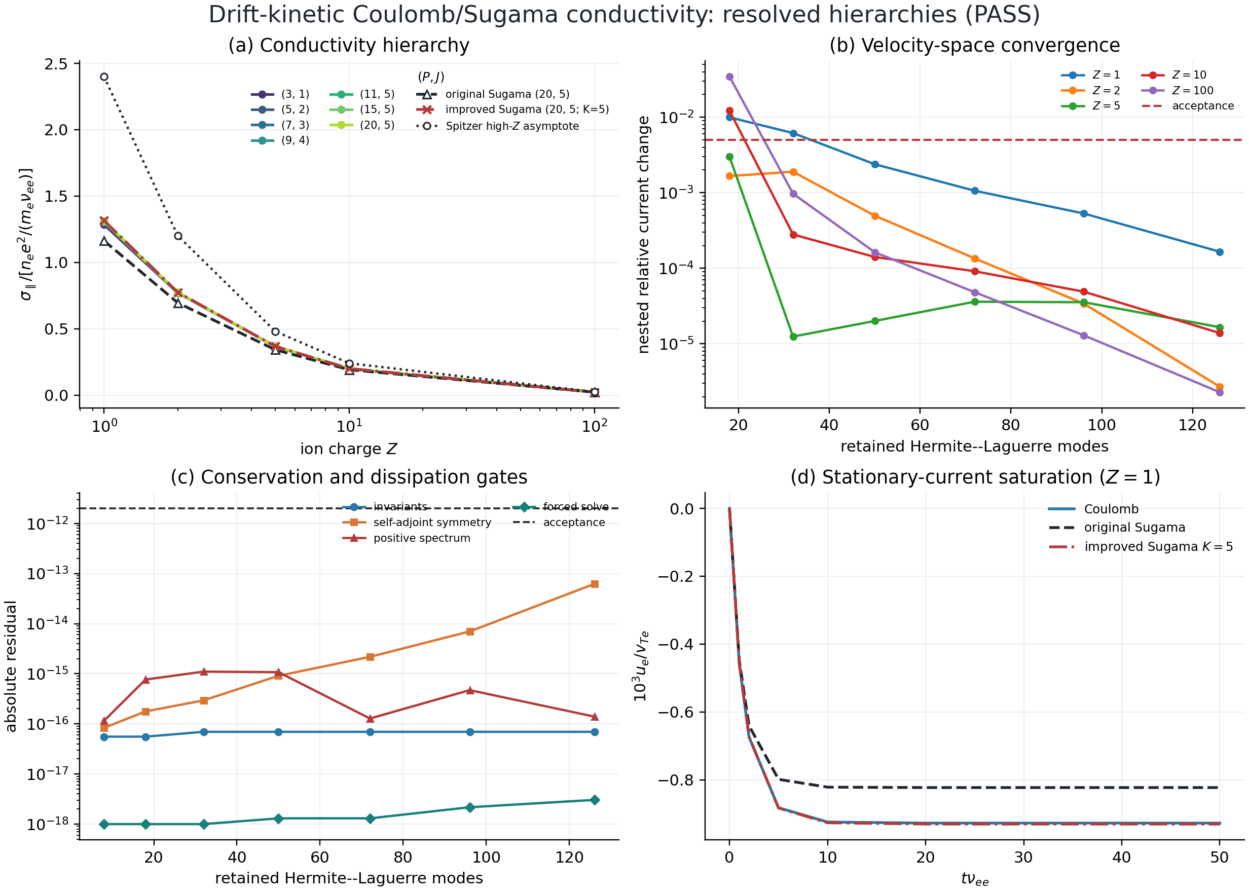
Drift-kinetic Coulomb and Sugama response hierarchies. Panel (a) compares Coulomb with the arbitrary-order original and improved models, panel (b) is the nested velocity-space error, panel (c) records the conservation and dissipation gates, and panel (d) reproduces stationary-current saturation at the paper’s applied-field normalization.
The machine-readable JSON and CSV use the same prospectively fixed 0.5% current and \(2\times10^{-12}\) algebra thresholds. At equal temperature, the arbitrary-order original-Sugama test matrix equals the Coulomb test matrix; its field matrix is the self-adjoint low-rank restoration of momentum and thermal energy. This construction reproduces every published C6 coefficient at low order and, at \((P,J)=(20,5)\), yields 11.29% less current than Coulomb at \(Z=1\) and only 0.61% less at \(Z=100\). Prospectively fixed gates require at least an 8% low-charge deficit and no more than a 2% high-charge difference, reflecting the Figure-16 ordering. The improved field correction is formed from the Coulomb Braginskii \(N\) matrix Schur complement and the exact drift-kinetic transforms in equations (79)–(81) of Frei, Ernst & Ricci (2022). It reproduces every C103 coefficient at \(K=1\); the shipped hierarchy retains complete total-degree shells through \(K=5\), checks the final \(K=4\rightarrow5\) response change, and requires agreement with Coulomb within 1% at every scanned charge. The measured maximum changes are 0.439% in the final correction-order step and 0.0237% from \((P,J)=(15,5)\) to \((20,5)\); the largest improved-to-Coulomb difference is 0.307%. Regenerate all three formats with
python tools/artifacts/build_linear_validation_artifacts.py collision-response
For the absolute normalization, define \(\widehat E=eE/(m_ev_{Te}\nu_{ee})\). The plotted response \((u_e/v_{Te})/\widehat E\) is then \(\sigma_\parallel/[n_e e^2/(m_e\nu_{ee})]\). The black curve in panel (a) is the Spitzer high-charge limit \(64/[3\,2^{3/2}\pi Z]\); the \(Z=100\) Coulomb point differs by 7.453%, inside the fixed 8% gate. Panel (d) uses the equivalent paper convention \(eE/(\sqrt{m_eT_e}\nu_{ee})=10^{-3}\). Its three exact matrix-exponential traces saturate by \(t\nu_{ee}=50\); independent steady solves over a 100x field range close the linear-response gate. These results promote the unmagnetized equal-temperature conductivity problem, not finite-\(b\) collisional transport.
A deterministic Cyclone ITG probe also records the finite-wavelength failure boundary rather than hiding it. At \(k_y\rho\simeq0.63\), increasing the normalized collision weight from zero to three damps the fitted growth rate; at \(k_y\rho\simeq0.94\), the same drift-kinetic model instead excites the short-wave branch. This is the behavior identified when collisional FLR terms are omitted in the local collisional-ITG study. The regression test therefore requires both observations and keeps configuration-file selection fail-closed. Only a finite-\(b\) operator may promote the short-wavelength lane.
The finite-\(b\) runtime path now has a shared multiprecision pair-table builder that amortizes wavelength-independent basis algebra and converts the paper’s Laguerre signs to the runtime convention. This is an implementation prerequisite, not the integrated ITG gate. A low-order \((P,J)=(3,1)\) development probe still excites the short-wave branch even with the complete finite-\(b\) contribution. Consistent with the paper’s convergence study, the result is rejected as velocity-space under-resolution. Increasing from \((3,1)\) to \((5,2)\) lowers its fitted collisional growth from 0.773 to 0.520, but does not suppress it. Promotion requires the independently converged \((18,6)\) endpoint and matching \(k_\perp\)/collisionality scans; no reduced probe or favorable trend substitutes for it.
Offline generation also factors the equation-(B5) associated-basis overlap exactly into a Gamma-weighted radial Laguerre contraction and a differentiated angular Legendre contraction, then reuses that overlap across each parity shell. At \((P,J)=(5,2)\), with two wavelengths, spherical/radial cutoffs 9/4, Bessel–Laguerre cutoff 6, and 32 decimal digits, this reduced wall time from 184.01 s to 26.41 s (7.0x) without changing the table checksum. This is a table-generation result, not a simulation or transport speedup claim. A higher \((P,J)=(7,3)\) two-wavelength table now completes serially in 411.22 s inside the external campaign bound. Its zero-wavelength test/field blocks agree with the independently generated drift-kinetic equations to relative errors \(1.08\times10^{-31}\) and \(1.92\times10^{-32}\). This is validated hierarchy evidence, but remains below the required \((18,6)\) ITG endpoint.
The equal-species original-Sugama finite-wavelength slice is now separate from that Coulomb field model. At equal mass and temperature, equations (3.72)– (3.76) of Frei et al. (2021) make its test component exactly the Coulomb test component. Equations (3.79) and (3.65), (3.68)–(3.69), and (3.80) make the field component the sum of three explicit rank-one parallel-flow, perpendicular-flow, and energy responses. The response vectors are projected directly with product velocity quadrature; they are not inferred by forcing finite-wavelength gyrocenter moments into the null space. The offline conversion reuses the expensive Coulomb test table:
python tools/artifacts/build_linear_validation_artifacts.py \
  collision-original-sugama-table \
  --coulomb-table finite_b_zonal_P24_J10_diagonal.npz \
  --out finite_b_zonal_P24_J10_original_sugama.npz \
  --quadrature-order 80
The archive conversion requires complete angular coverage, the signed runtime
Laguerre convention, finite coefficients, and agreement between 80- and
96-node projections. Its equation test reproduces the published drift-kinetic
C6 construction at \(B=0\) to roundoff and limits the finite-wavelength
field block to a symmetric rank-three matrix. At finite \(B\), the flow
channels have the nonzero gyro-diffusive action required by the gyroaveraged
operator, while the symmetric part of the complete retained collision matrix
remains strictly dissipative in the equation-level gate.
EqualSpeciesFiniteWavelengthSugamaOperator
interpolates the resulting table in JAX and acts on the post-field
nonadiabatic response \(H\); JIT/JVP and finite-difference interpolation
gates pass, but a paper-facing zonal trace is still required for promotion.
The finite-wavelength improved-Sugama field correction is generated from the same Coulomb archive. At equal mass and temperature the test correction vanishes, while equations (61)–(69) of Frei, Ernst & Ricci (2022) add the Braginskii field correction through parallel and perpendicular generalized flow projections. The implementation evaluates those velocity integrals independently with product Gauss–Hermite/Laguerre quadrature and accepts the higher-order result only when an additional 16 nodes change the correction by less than \(10^{-11}\) relative or \(10^{-12}\) absolute:
python tools/artifacts/build_linear_validation_artifacts.py \
  collision-improved-sugama-table \
  --coulomb-table finite_b_zonal_P24_J10_diagonal.npz \
  --out finite_b_zonal_P24_J10_improved_sugama.npz \
  --correction-order 5 --quadrature-order 80 --digits 80
At \(B=0\), correction orders \(K=1,2,3\) reproduce the independent drift-kinetic analytical implementation with relative matrix errors from \(3.4\times10^{-15}\) to \(1.1\times10^{-14}\). At the production P24/J10, \(K=5\) resolution, nested 80/96-node checks over \(B=0.12,0.16,0.24,0.32\) differ by at most \(7.1\times10^{-14}\) relative. These are equation and quadrature gates. The Figure-13/14 zonal ordering and velocity-section comparison is the independent physical gate; it now passes at P24/J10 through \(t\nu=30\). At \(k_x\rho_i=0.1\), the late responses are 0.00242 (original), 0.00255 (improved), and 0.00288 (Coulomb); at \(k_x\rho_i=0.2\), they are \(9.66\times10^{-5}\), \(1.15\times10^{-4}\), and \(1.92\times10^{-4}\) in the same order. The improved early-window RMS error relative to Coulomb is lower than the original-model error at both wavenumbers. The common finite-wavelength runner now accepts provenance-matched Coulomb, original-Sugama, and improved-Sugama archives. For the \(k_x=0.2\) trace it can checkpoint the physical \(t\nu=5\) state, reconstruct the equation-(52) parallel and perpendicular gyrocenter-distribution cuts at the outboard midplane, and continue the same integration to \(t\nu=30\).
As a separate full-distribution reference utility,
conservative_full_f_dougherty_cross_moments. For directed collision rates
\(\nu_{sr}\), it evaluates the pairwise primitive moments
These are equations (2.11)–(2.12) of the improved multispecies Dougherty derivation. Francisquez et al. derive a nonlinear full-\(f\) Fokker–Planck model, whereas GKX evolves a linearized delta-\(f\) gyrokinetic state. The JAX implementation accepts arbitrary mass ratios and directed rates, keeps zero-rate and self pairs unchanged, and is equation-gated for pairwise momentum and energy conservation, the equal-species limit, positive target temperature, and AD/finite-difference agreement. A three-species, multi-sample gate also checks every interacting pair for \(d_v=1,2,3\) and verifies Galilean invariance of the target flow and thermal speed. It supports derivation checks and future full-\(f\) work; it must not be inserted directly into the shipped linearized field-particle restoration.
The next runtime model tier extends this verified low-order normalization to the published linearized gyrokinetic Sugama/Coulomb operators in the full Hermite–Laguerre moment basis. A linearized multispecies Dougherty variant is admissible only after its delta-\(f\) projection is derived explicitly; the full-\(f\) primitive targets are not used as a shortcut. Promotion requires discrete Maxwellian null-space, particle conservation per species, total momentum and energy conservation, adjointness, non-positive entropy production, velocity-resolution convergence, collisional ITG, conductivity, and zonal-flow damping gates.
Relevant derivations and verification targets include the Laguerre–Hermite pseudo-spectral formulation, the advanced linearized gyrokinetic moment operators, the improved Sugama moment implementation, and the local collisional ITG study. The independent GYACOMO source implementation loads full Sugama/Landau test and field matrices generated offline by COSOlver, interpolates them in \(k_\perp\), and applies the dense moment coupling at runtime. That audit supports the same separation here: generate cancellation-sensitive coefficients in high precision, store provenance and checksums, then keep the JAX runtime to validated table interpolation and matrix application.
Controls:
RuntimePhysicsConfig.collisionsRuntimeTermsConfig.collisionsRuntimeSpeciesConfig.nuRuntimeCollisionConfig.nu_hermiteRuntimeCollisionConfig.nu_laguerre
For two kinetic species, the explicit species-parallel integrator evaluates
this complete collision contribution locally on each device after the shared
field reduction. Nonzero, unequal ion/electron rates are identity-gated against
serial RHS evolution on logical CPUs and two office GPUs. The direct
species-sharded RHS helper remains collision-free; use
integrate_linear(..., parallel=RuntimeParallelConfig(strategy="velocity",
axis="species", num_devices=2))
for the validated collisional route.
The guiding-centre invariant gate is explicitly long-wavelength. At \(k_\perp\rho=0\), a five-step gate starts from populated high moments, requires a nonzero collision response, and preserves each species’ density, parallel-momentum, and temperature-like moments in both serial and decomposed integration. At finite \(k_\perp\rho\), guiding-centre density, momentum, and energy are not locally conserved; collisions are local in real space, and the gyrocentre change is nonlocal. This is physical behavior of the published model, not a residual to tune away. A direct finite-\(b\) gate checks every term of equations (3.38)–(3.42), including parallel/perpendicular flow and temperature restoration. Promotion to Landau/Sugama remains blocked because those operators contain different velocity-dependent test-particle and species-coupled field-particle physics, not because this model should be forced to conserve finite-\(b\) guiding-centre moments.
The same enclosing route is gated for Hermite/Laguerre hypercollisions with
explicitly populated high moments and nonzero nu_hyper_l/nu_hyper_m.
This verifies that the decomposed operator damps its intended high-order
subspace while retaining serial evolution identity; it is separate from the
low-order conserving collision correction above.
Electromagnetic species decomposition reuses the serial field equations rather
than maintaining a second approximation. Local density, parallel-current,
polarization, and perpendicular-pressure moments are summed over the local
species axis and then reduced across the named device axis. The resulting
phi, apar, and bpar are shared by each local RHS assembly. A
two-species gate requires nonzero magnetic fields and serial/decomposed
trajectory identity; it does not yet cover mixed species–Hermite meshes.
Hypercollisions
GKX implements three Hermite/Laguerre hypercollision branches and an optional \(|k_z|\)-scaled branch:
Controls:
RuntimePhysicsConfig.hypercollisionsRuntimeTermsConfig.hypercollisionsRuntimeCollisionConfig.nu_hyperRuntimeCollisionConfig.nu_hyper_lRuntimeCollisionConfig.nu_hyper_mRuntimeCollisionConfig.nu_hyper_lmRuntimeCollisionConfig.p_hyperRuntimeCollisionConfig.p_hyper_lRuntimeCollisionConfig.p_hyper_mRuntimeCollisionConfig.p_hyper_lmRuntimeCollisionConfig.hypercollisions_constRuntimeCollisionConfig.hypercollisions_kz
Hyperdiffusion And End Damping
The perpendicular hyperdiffusion term is
masked by the dealias region.
The field-line end damping is
Controls:
RuntimeTermsConfig.hyperdiffusionRuntimeCollisionConfig.D_hyperRuntimeCollisionConfig.p_hyper_kperpRuntimeCollisionConfig.damp_ends_ampRuntimeCollisionConfig.damp_ends_widthfracRuntimeCollisionConfig.damp_ends_scale_by_dt
Nonlinear \(E \\times B\) And Flutter
The nonlinear bracket is evaluated pseudospectrally:
The electrostatic nonlinear term is
and the electromagnetic flutter contribution couples adjacent Hermite moments:
Controls:
TimeConfig.compressed_real_fftTimeConfig.laguerre_nonlinear_modeTimeConfig.nonlinear_dealiasRuntimeTermsConfig.nonlinear
Source Mapping
linear term kernels:
src/gkx/terms/linear_terms.pynonlinear term kernels:
src/gkx/terms/nonlinear.pyassembly:
src/gkx/terms/assembly.pylow-level parameter container:
src/gkx/linear.pyruntime parameter surface:
src/gkx/workflows/runtime/config.py
Parameter Surface
The primary parameter groups are:
RuntimePhysicsConfigRuntimeCollisionConfigRuntimeNormalizationConfigRuntimeTermsConfigLinearParams
For TOML syntax and all supported keys, see Input Files and Executable.