Performance

JAX performance model

Current-branch representative refresh

The compact refresh in benchmarks/references/gkx_2_representative_performance_refresh.json admits two bounded local-CPU rows after finite CPU/GPU numerical checks. The matching office-GPU timings are retained as rejected provenance because both A4000s were already at 100% utilization; they do not update the published speed claim. An uncontended rerun is required before replacing the historical GPU panel.

GKX uses JAX to compile array kernels ahead of time, enabling vectorized, accelerator-ready performance while retaining automatic differentiation. The linear operator and time integrator are designed to be jit-friendly and to avoid Python-side loops in performance-critical paths.

The linear solver precomputes geometry-dependent arrays (gyroaverage coefficients, drift components, mirror term, and zero-mode masks) in a LinearCache to avoid recomputing them at each time step. This cache is reused inside the JIT compiled integrator.

Cache profiling

Cache profiling uses the maintained cache-build subphase profiler, not the old cached-versus-uncached local timing probe. The profiler decomposes build_linear_cache() into geometry loading, spectral-grid construction, gyroaverages, Laguerre transforms, drift coefficients, damping factors, and the final cache assembly. This makes performance work actionable because each row maps to a concrete cache-construction phase.

python tools/profiling/profile_startup_and_cache.py linear-cache \
  --config examples/nonlinear/axisymmetric/runtime_cyclone_nonlinear.toml \
  --Nl 4 --Nm 8 \
  --json-out tools_out/linear_cache_cyclone_gpu.json \
  --csv-out tools_out/linear_cache_cyclone_gpu.csv

Fixed-step linear integrator profiling

Use the maintained integrator benchmark for matched warm fixed-step profiles; it accepts explicit method, timestep, resolution, and JSON-output controls:

python benchmarks/performance/benchmark_integrators.py \
  --skip-diffrax --method sspx3 --steps 480 --dt 0.005 \
  --Nl 7 --Nm 14 --ky 0.3 --warmup 1 --repeat 5 \
  --out-json tools_out/linear_sspx3_profile.json

The tracked before/after artifact docs/_static/linear_sspx3_stage_profile.json compares the same finite Cyclone trajectory before and after explicit-stage consolidation. State and field-history norms agree exactly, while median CPU times are 3.202 s and 3.223 s. The 0.7% difference is below the 3% reporting threshold and has the wrong sign for a speedup claim. XLA already removed the unused SSPX3 stage from the compiled graph; the change therefore improves single ownership and eager execution without a measurable end-to-end compiled speedup.

No speedup claim should be made from a local profile, scaling panel, or parallelization artifact unless the matching numerical-identity gate and hardware-specific profiler artifact are cited together. Current production parallelization claims are limited to independent-work batching; whole-state nonlinear sharding and nonlinear domain decomposition remain diagnostic unless their workload-specific identity and profiler promotion gates pass.

The nonlinear spectral-domain profile now records both the older global-reconstruction logical route and a pencil-FFT fused-bracket route. The pencil work model removes the state/bracket allgather from the estimated communication path and predicts plausible scaling on the tracked four-tile micro-route, but the local JIT timing remains below the production 1.5x gate. Treat this as implementation evidence for the next distributed-FFT tranche, not as a shipped nonlinear domain-decomposition speedup.

The follow-up z-sharded fused pencil RHS artifact docs/_static/nonlinear_device_z_pencil_rhs_cpu4_profile.json is the first active device-sharded version of that idea. It passes serial-vs-sharded RHS identity on a (4,16,96,96,32) bracket workload with maximum absolute error 7.6e-10. The shard_map route is now a CPU speedup candidate for this RHS microkernel: 1.51x on two logical CPU devices and 2.62x on four logical CPU devices. The two-GPU office artifact docs/_static/nonlinear_device_z_pencil_rhs_gpu2_profile.json also passes host-gathered RHS identity (max_abs_error=5.24e-10) after staging the initial state through host before applying explicit z sharding, but reaches only 1.09x versus the single-GPU serial JIT route, below the 1.5x GPU speedup gate.

The next gate is a fixed-step physical transport-window profile that advances the same serial and z-sharded routes for four nonlinear steps and compares the final state plus free-energy, field-energy, physical-flux, and bracket-RMS traces. The CPU artifact docs/_static/nonlinear_device_z_pencil_transport_cpu4_profile.json passes all active identity checks on two and four logical CPU devices for the same (4,16,96,96,32) workload. It reaches 1.61x on two logical CPU devices and 3.13x on four, with maximum final-state absolute error 7.45e-9. The HLO dump recorded in the JSON shows local FFT lowering for the sharded route and no all-to-all or collective-permute operations. The matching two-GPU artifact docs/_static/nonlinear_device_z_pencil_transport_gpu2_profile.json also passes the transport-window identity gate (max_abs_error=7.45e-9), but only reaches 1.48x versus one GPU. Its Perfetto/TensorBoard trace was written under /tmp/gkx_traces during generation, and its HLO summary likewise shows no collectives. The GPU blocker is therefore speedup/work granularity, not numerical identity or a hidden global reconstruction. This remains a micro-route transport-window claim, not a full production nonlinear turbulence-solve speedup claim.

For larger GPU diagnostic grids, the profiler also supports --z-chunk-size or --auto-z-chunk-size. The automatic option uses a backend-free cuFFT batch-pressure preflight model to choose a local z_chunk_size before launching the timed route. This processes independent local z slabs separately and can avoid cuFFT batched-plan failures when used with XLA_PYTHON_CLIENT_PREALLOCATE=false. The June 13, 2026 office diagnostics used this mode to run previously failing (4,16,96,96,64) and (4,16,128,128,32) transport windows, but their two-GPU speedups were only about 1.40x and 1.30x respectively. Treat this as bottleneck localization, not as promotion evidence.

Use --observable-repeats when a device-z transport-window profile needs to separate compute-only RHS/integrator timing from the scalar observable and identity-gate path. The speedup rows still time only fixed-step final-state updates; the observable_gate_* JSON/CSV fields report the cost of host-gathered free-energy, field-energy, physical-flux, and bracket-RMS checks separately. Those fields are diagnostic bottleneck evidence and are not part of the nonlinear speedup promotion gate. Use --observable-mode sharded_reduce to evaluate the same scalar observables through z-sharded device reductions instead of full-state host gathers. This is an identity/profiling option, not a production speedup mode: when it recomputes the nonlinear bracket only for diagnostics, it can be slower than the host-gathered path. A production version should fuse scalar diagnostic accumulation into the RHS/update route rather than launching a second bracket pipeline. The tracked office artifact docs/_static/nonlinear_device_z_pencil_transport_gpu2_observable_split_profile.json records this split on the (4,16,96,96,64) auto-chunked two-GPU diagnostic: identity passes, compute-only speedup remains below gate at 1.19x, and the observable gate median is about 42.6 times the sharded compute median. The next production route should therefore keep scalar diagnostics streamed and fused with the device computation rather than host-gathering full states or recomputing the nonlinear bracket every step.

For this release, performance work is closed at that evidence-backed boundary: runtime/memory accounting, nonlinear RHS hot-path localization, production independent-work parallelization, and diagnostic nonlinear decomposition identity are tracked and reproducible. Production nonlinear domain decomposition is deferred until a full solver route fuses scalar diagnostics into the RHS/update path and clears matched CPU/GPU transport-window speedup gates.

Nonlinear profiling

For end-to-end nonlinear performance, use the dedicated Cyclone profiling driver. It supports Perfetto traces, XLA HLO dumps, and memory snapshots.

python tools/profiling/profile_runtime_kernels.py cyclone \
  --trace-dir /tmp/gkx_nl_trace \
  --xla-dump-dir /tmp/gkx_nl_xla \
  --steps 400 --dt 0.0377 --Nl 4 --Nm 8

For repeated Python objective or ensemble calls with fixed geometry and model policy, add --reuse-prepared-simulation and an explicit --steps. The ordinary command remains the executable-style end-to-end startup profile; the prepared mode measures compile-once repeated-call throughput.

The trace directory can be opened with Perfetto. For GPU profiling, set JAX_PLATFORM_NAME=gpu before invoking the script. JAX writes the trace under <trace-dir>/plugins/profile/<timestamp>/*.trace.json.gz together with the corresponding *.xplane.pb metadata; the same directory can be opened in XProf, while the optional memory.prof snapshot can be inspected with pprof or XProf’s memory tooling.

JAX/XProf operational notes

Two JAX runtime details matter when reading short-run performance numbers:

• JAX’s persistent compilation cache can remove repeated recompilation cost for fixed signatures. For repeated local profiling runs, set JAX_COMPILATION_CACHE_DIR before the first compilation. This is useful for engineering sweeps, but the shipped runtime panel should remain a cold end-to-end measurement unless stated otherwise.

• JAX GPU runs preallocate most device memory by default. When diagnosing an out-of-memory failure on a shared machine, use XLA_PYTHON_CLIENT_PREALLOCATE=false or a reduced XLA_PYTHON_CLIENT_MEM_FRACTION during the profiling run. Those knobs are useful for debugging and tracing, but they should not silently change the published benchmark contract.

Recent nonlinear profiling (Cyclone, benchmark-locked config)

Reference run configuration (March 4, 2026):

• ky=0.3, Nl=4, Nm=8

• dt=0.01, steps=400

• sample_stride=10, diagnostics_stride=10

• tools/profiling/profile_runtime_kernels.py cyclone with the tracked Cyclone runtime config

CPU profiling (Apple CPU, JAX CPU backend):

warmup_time_s=117.803
run_time_s=109.147

GPU profiling (A100-class GPU, JAX CUDA backend):

warmup_time_s=38.950
run_time_s=21.350

HLO summary (jit_scan.*_after_optimizations):

• CPU: fft=623, scatter=72, gather=375, dot=88, fusion=1053

• GPU: fft=440, scatter=30, gather=322, dot=44, fusion=831

The nonlinear RHS remains FFT-heavy with nontrivial gather/scatter density. Primary optimization targets are the FFT pipeline (channel stacking, reuse of real-space gradients) and scatter removal in linked-FFT paths.

GPU memory report (jit_scan module):

• Total bytes used: 228.21 MiB (XLA memory usage report).

Nonlinear benchmark harness

To capture per-step runtime and end-of-run diagnostics, use the nonlinear benchmark harness:

python benchmarks/performance/benchmark_nonlinear_suite.py --steps 200 --dt 0.0377 \
  --out /tmp/gkx_nl_bench.csv

The harness records scalar diagnostics through the compact diagnostics path, so it measures runtime without materializing mode-resolved history arrays unless a separate publication artifact explicitly requests them.

To test the optional spectral nonlinear mode (no Laguerre quadrature grid):

python benchmarks/performance/benchmark_nonlinear_suite.py --laguerre-mode spectral

You can optionally pass a reference-code log file to compare runtime per step:

python benchmarks/performance/benchmark_nonlinear_suite.py --gx-log /path/to/gx_run.out

RHS kernel profile (nonlinear Cyclone)

The RHS split profiler measures field solve, nonlinear bracket, linear RHS, and full RHS kernels after compilation:

python tools/profiling/profile_runtime_kernels.py nonlinear-step-split \
  --config examples/nonlinear/axisymmetric/runtime_cyclone_nonlinear_short.toml \
  --repeats 10 \
  --out docs/_static/nonlinear_rhs_profile_gpu.csv

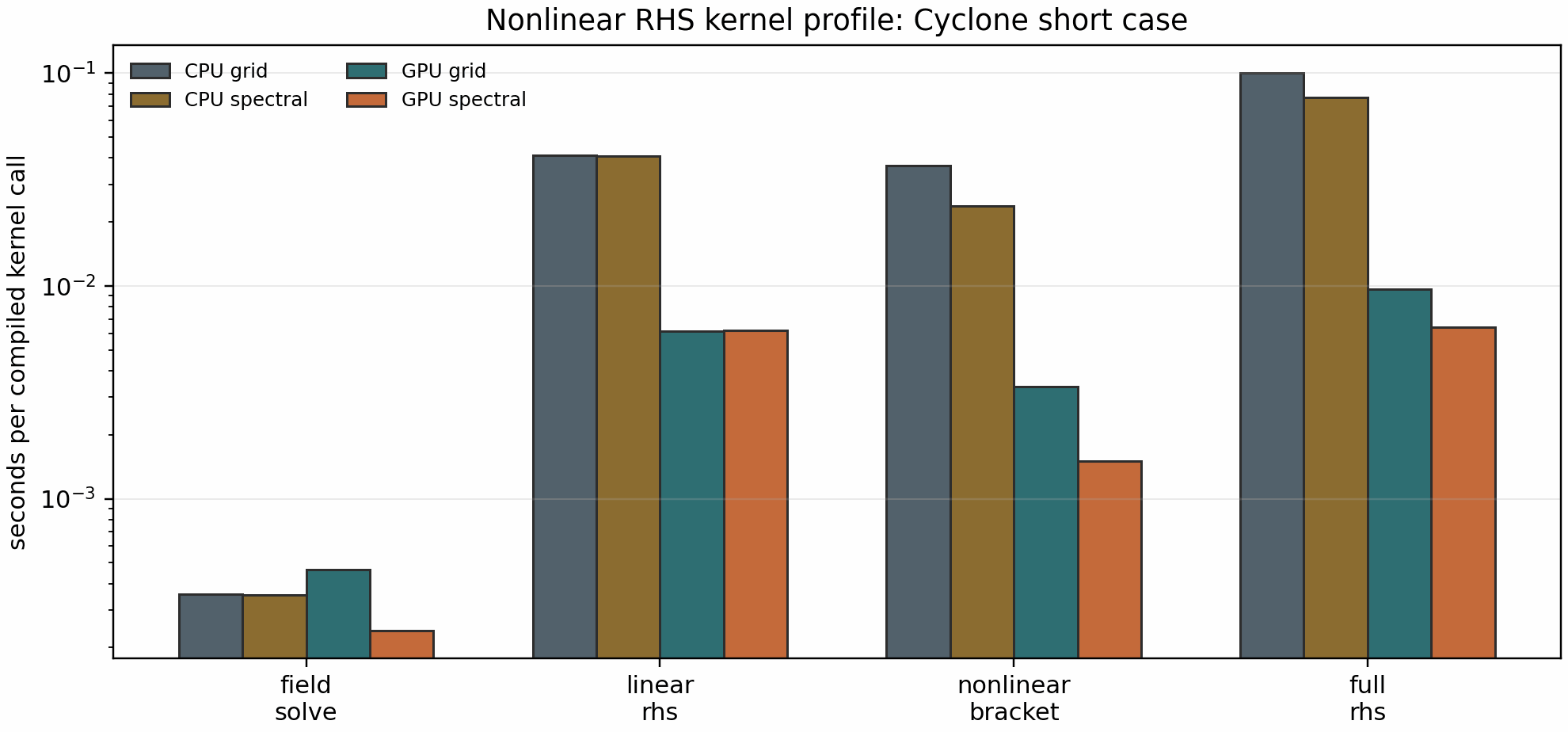
The current bounded Cyclone profile separates CPU and office GPU timings for default grid-mode and optional spectral-mode nonlinear brackets. The machine-readable companion docs/_static/nonlinear_rhs_profile.json records the dominant measured kernel, kernel fractions relative to the full RHS, and grid-to-spectral speedups for each backend. The May 9, 2026 refresh used the same short-case 10-repeat harness on local CPU and one office RTX A4000 with CUDA_VISIBLE_DEVICES=0 after the linear-RHS fast-path and linked-FFT refactor tranche. The GPU environment reported jax==0.6.2/jaxlib==0.6.2; these are profiler-local hot-path measurements, not a broad production runtime claim. The refreshed GPU grid-mode split is:

python tools/artifacts/plot_scaling_panels.py rhs-profile \
  --out docs/_static/nonlinear_rhs_profile.png

field_solve=4.65e-4 s
nonlinear_bracket=3.36e-3 s
linear_rhs=6.13e-3 s
full_rhs=9.66e-3 s

The same GPU profile with laguerre_mode="spectral" measured nonlinear_bracket=1.50e-3 s and full_rhs=6.38e-3 s. CPU full-RHS timings from the same harness were 1.01e-1 s for grid mode and 7.73e-2 s for spectral mode. The short-harness spectral full-RHS ratios are now 1.30 on CPU and 1.51 on GPU for this Cyclone case, while the nonlinear-bracket-only ratios are 1.54 on CPU and 2.24 on GPU. The spectral mode therefore remains an opt-in mode guarded by the case-level parity gate below rather than a global default.

The dominant remaining warm-throughput cost is the compiled linear RHS, with the nonlinear FFT pipeline still relevant for larger production grids. The next performance step is to repeat this split on larger benchmark-size cases and then use profiler traces to decide whether fusion, layout changes, or production decomposition give the largest verified win.

Benchmark-size Cyclone Miller RHS profile

The larger Cyclone Miller profile uses the shipped nonlinear Miller input with Nx=192, Ny=64, Nz=24, Nl=4, and Nm=8. This is still a single compiled-RHS split profile rather than a full transport-average runtime claim, but it is large enough to expose a different bottleneck balance than the short Cyclone case.

python tools/profiling/profile_runtime_kernels.py nonlinear-step-split \
  --config examples/nonlinear/axisymmetric/runtime_cyclone_nonlinear_miller.toml \
  --repeats 5 \
  --out docs/_static/nonlinear_rhs_profile_miller_cpu.csv

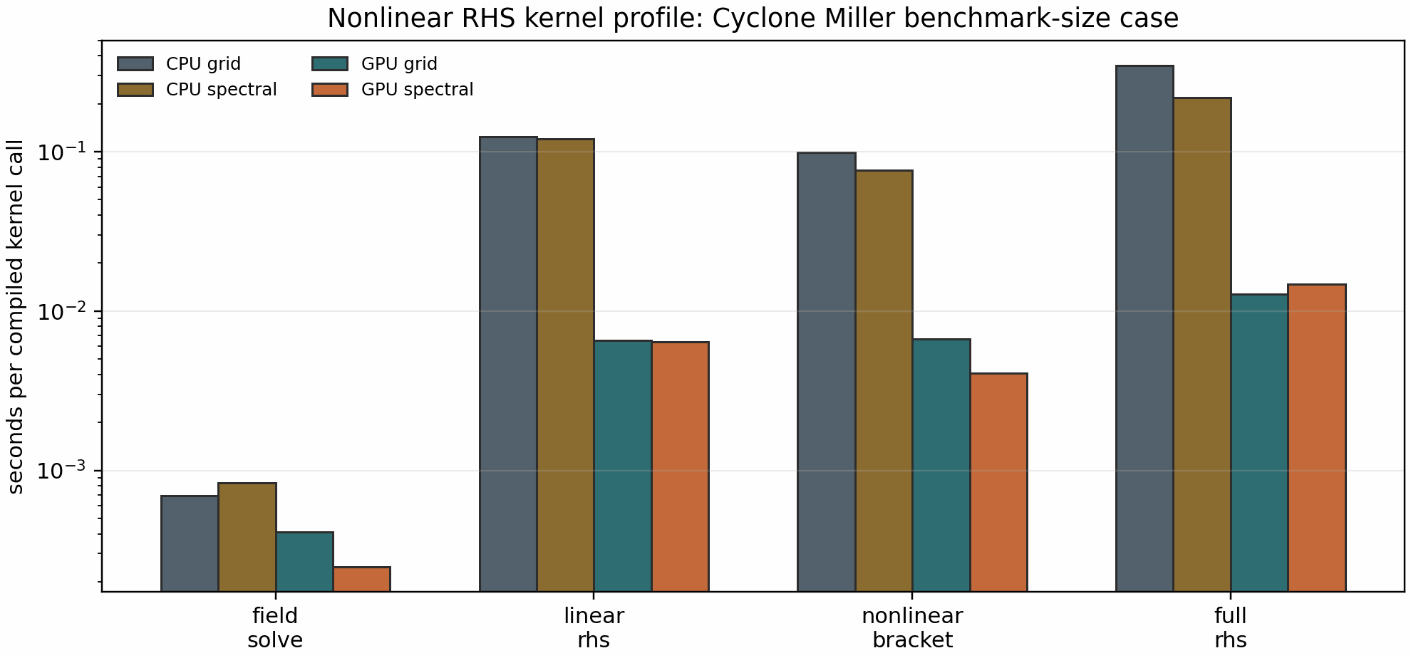
The May 10, 2026 local CPU refresh after the independent-worker parallelization tranche measured CPU full-RHS timings of 3.48e-1 s in grid mode and 2.20e-1 s in spectral Laguerre mode, with measured sub-kernels linear_rhs=1.24e-1 s and nonlinear_bracket=9.89e-2 s in grid mode. On one office RTX A4000, the tracked artifact still records corresponding full-RHS timings of 1.28e-2 s and 1.48e-2 s. Spectral mode reduces the GPU nonlinear bracket by 1.63x, but the full GPU RHS remains faster in grid mode because the optimized Laguerre transform removes enough layout overhead while preserving the production grid-quadrature convention. The CPU refresh continues to point the next optimization pass at linear-RHS fusion/cache layout and larger-grid bracket decomposition, not at claiming a broad nonlinear speedup from spectral mode alone.

The full fused nonlinear-RHS trace companion is generated with:

python tools/profiling/profile_runtime_kernels.py full-nonlinear-rhs \
  --config examples/nonlinear/axisymmetric/runtime_cyclone_nonlinear_miller.toml \
  --ky 0.3 \
  --Nl 4 \
  --Nm 8 \
  --repeats 5 \
  --summary-json docs/_static/full_nonlinear_rhs_trace_summary.json

The tracked local CPU artifact docs/_static/full_nonlinear_rhs_trace_summary.json reports warm_seconds=3.35e-1 and 3343 HLO lines. The matched one-RTX-A4000 artifact docs/_static/full_nonlinear_rhs_trace_gpu_summary.json reports warm_seconds=1.28e-2 and 3336 HLO lines. The GPU token triage is dominated by reshapes (1545), broadcasts (1822), multiplies (871), FFTs (229), slices (215), and reductions (132). This confirms that the next nonlinear performance tranche should target fused layout and bracket data movement rather than claiming a new runtime speedup from the linear-RHS specialization alone. The same tranche removed a duplicated non-Laguerre field mask from the nonlinear bracket path and then replaced the Laguerre-grid moveaxis/tensordot/moveaxis transforms with precision-controlled einsum calls. Transform-only CPU/GPU probes showed exact agreement with the previous algebra at the tested precision; on one RTX A4000 the full fused nonlinear-RHS trace improved from 1.49e-2 s to 1.28e-2 s while transposes dropped from 44 to 32. This is a bounded profiler-state source improvement, not a full transport runtime claim.

Runtime-mode stellarator RHS smoke profile

The release-performance gate also tracks W7-X and HSX at their documented adiabatic-electron nonlinear runtime mode (Nx=96, Ny=96, Nz=48, Nl=4, Nm=8, and the runtime k_y=1/21). These are not full transport-average timings; they are single-state RHS split profiles used to verify that the optimized grid-Laguerre path, VMEC/EIK geometry inputs, and CPU/GPU hot-path accounting remain consistent on non-axisymmetric cases.

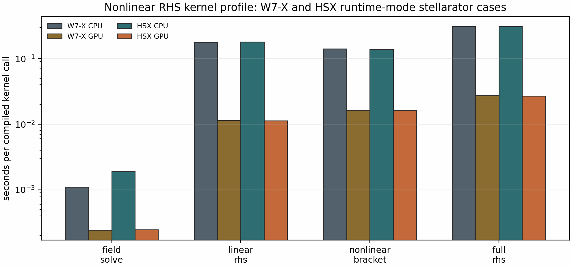
The tracked artifact docs/_static/nonlinear_rhs_profile_stellarator_runtime.json reports W7-X CPU/GPU full-RHS timings of 3.09e-1 s and 2.73e-2 s and HSX CPU/GPU full-RHS timings of 3.09e-1 s and 2.71e-2 s. In both stellarator runtime-mode profiles the GPU row is dominated by the nonlinear bracket (~59-60% of the measured full RHS), with the linear RHS contributing ~42%. That closes the release-level performance evidence: CPU/GPU profiler artifacts are current, the sharding identity gate is tracked, and the documentation makes only bounded profiler claims. Further nonlinear speedup work should target larger-state bracket/linear-RHS layout and must keep using identity gates before any production runtime claim.

Linear RHS term profile

The linear RHS split profiler drills into the compiled linear contribution used inside nonlinear runs:

python tools/profiling/profile_linear_rhs_terms.py \
  --config examples/nonlinear/axisymmetric/runtime_cyclone_nonlinear.toml \
  --ky 0.3 \
  --Nl 4 \
  --Nm 8 \
  --repeats 8 \
  --out docs/_static/linear_rhs_terms_profile_cpu.csv \
  --summary-json docs/_static/linear_rhs_terms_profile.json

After the zero-collision fast path and linked-FFT refactor, the May 9, 2026 CPU Cyclone artifact reports full_linear_rhs=1.08e-1 s for the compiled full linear RHS call in this profiling harness. The independently timed term kernels sum to 1.68e-2 s; this remaining gap is a localization signal, not a speedup claim, because the full path recomputes the field solve, H assembly, and all weighted contributions as one compiled graph. The largest standalone terms are hypercollisions (2.39e-3 s), linked |k_z| setup (2.38e-3 s), and streaming (2.34e-3 s). The accepted zero-collision branch now costs 1.11e-3 s in the standalone CPU timing and is guarded by the state-window identity gate below.

The active-state CPU companion docs/_static/linear_rhs_terms_profile_z_wave_cpu.json profiles the same state after injecting a resolved parallel perturbation. There the hypercollision and linked |k_z| norms are both 2.35e-4 and the linked |k_z| path costs 2.33e-3 s on CPU. This is the artifact that should be used for linked-|k_z| optimization decisions; the initial-state profile is only a zero-source baseline.

For the larger Cyclone Miller benchmark-size RHS profile above, the active-state CPU companion is docs/_static/linear_rhs_terms_profile_miller_cpu.json. It uses the same Nl=4, Nm=8, k_y=0.3 state as the nonlinear Miller profiler and reports full_linear_rhs=2.93e-1 s with independently timed terms summing to 4.83e-2 s. The largest nonzero standalone row is streaming (7.33e-3 s), followed by linked \partial_z (6.39e-3 s), linked |k_z| (6.18e-3 s), and hypercollisions (6.20e-3 s). That keeps the next bounded optimization focused on full-graph layout/fusion and reusable state transforms rather than making a standalone-term speedup claim.

The matching office GPU profile is tracked in docs/_static/linear_rhs_terms_profile_gpu.json and docs/_static/linear_rhs_terms_profile_gpu.csv. On one RTX A4000 with the same jax==0.6.2/jaxlib==0.6.2 environment used for the nonlinear RHS refresh, it reports full_linear_rhs=5.50e-3 s and independently timed terms summing to 3.41e-3 s. The accepted zero-collision branch costs 1.24e-4 s in the standalone GPU timing; hypercollisions and linked |k_z| remain present as separately profiled rows. The active-state GPU companion docs/_static/linear_rhs_terms_profile_z_wave_gpu.json activates the same operator pair with matched norms 2.35e-4 and records linked |k_z| at 3.63e-4 s with full_linear_rhs=5.48e-3 s.

The companion state-window gate is generated with:

python tools/artifacts/generate_linear_rhs_parallel_gates.py zero-norm-state-window \
  --config examples/nonlinear/axisymmetric/runtime_cyclone_nonlinear.toml \
  --ky 0.3 \
  --Nl 4 \
  --Nm 8 \
  --out-json docs/_static/linear_rhs_zero_norm_state_window_gate.json

The current gate passes by accepting the zero-collision skip for this nu=0 Cyclone window while rejecting a hypercollision skip: the initial state has zero relative hypercollision skip error, but the resolved z-varying state reaches 3.59e-3. This protects the optimization path from incorrectly disabling linked |k_z| hypercollisions based only on the initial-state profile.

Full fused linear RHS trace

The term profiler above times independently isolated kernels. The companion full-graph profiler lowers and times the production linear_rhs_cached entry point for a real runtime TOML so optimization work can target the compiled graph seen by executable linear runs rather than only the standalone assembly helper:

python tools/profiling/profile_runtime_kernels.py full-linear-rhs \
  --config examples/nonlinear/axisymmetric/runtime_cyclone_nonlinear_miller.toml \
  --ky 0.3 \
  --Nl 4 \
  --Nm 8 \
  --repeats 3 \
  --summary-json docs/_static/full_linear_rhs_trace_summary.json

The May 11, 2026 local CPU production-path artifacts record source="gkx.operators.linear.rhs.linear_rhs_cached" and force_electrostatic_fields=true. The initial-state companion reports warm_seconds=1.54e-1 and compile_execute_seconds=1.02. The active z_wave companion injects resolved parallel variation and reports warm_seconds=8.38e-2 with the same specialized HLO shape. Both summaries contain 2779 HLO lines and highlight the remaining graph-level pressure points: broadcasts (983 coarse token hits), reshapes (578), FFT mentions (312), reductions (316), multiplies (200), and gathers (51). These are localization metrics, not standalone runtime claims. The source-path change means these artifacts should be compared against future production-path refreshes, not against older lower-level assembly-helper artifacts.

The May 11, 2026 one-RTX-A4000 production-path artifacts docs/_static/full_linear_rhs_trace_gpu_summary.json and docs/_static/full_linear_rhs_trace_gpu_z_wave_summary.json report source="gkx.operators.linear.rhs.linear_rhs_cached", 2779 HLO lines, and force_electrostatic_fields=true. The initial and active z_wave states measure warm_seconds=5.13e-3 and 5.15e-3, respectively. These GPU artifacts show that the production linear-RHS path remains about five milliseconds on one RTX A4000 for this benchmark-size RHS call, but they remain kernel-localization evidence rather than a full nonlinear runtime claim.

Parallelization scaling guardrail

The earlier two-device linear scaling figure remains an engineering artifact, not the headline production parallelization claim. Current user-facing scaling claims should point to the independent k_y scan and quasilinear/UQ ensemble figures below, because those paths preserve serial ordering and have explicit solver-observable identity gates.

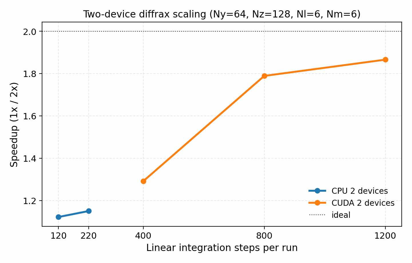
The raw sweep data lives in docs/_static/scaling_speedup_data.csv and can be replotted with:

python tools/artifacts/plot_scaling_panels.py diffrax-speedup

The exploratory distributed-RK2 strong-scaling data is still tracked for engineering work, but it is intentionally not presented as a headline publication figure because the current curve is dominated by communication overhead rather than near-ideal scaling.

Production parallelization should start with independent work rather than nonlinear domain decomposition. The public helpers gkx.ky_scan_batches and gkx.batch_map split k_y scans, quasilinear/UQ ensembles, and sensitivity-sweep workloads while preserving serial ordering. On one device they reduce to batched vmap execution; on multiple devices they use JAX device batching and trim padded edge samples deterministically. Every performance claim from this path should include a numerical-identity gate against the serial result before a speedup plot is promoted.

For the release-scale CPU/GPU panels below, the acceptance contract is machine-checkable: the combined *_large artifact must cite split CPU and GPU JSON/CSV/PNG/PDF companions, each split artifact must include the grid, warmup/repeat policy, backend/device counts, positive timing samples, and per-row identity results, and any speedup statement must name the artifact that supports it. Whole-state nonlinear sharding uses the same large-run artifact shape, but its timing ratios remain profiler evidence and not a production nonlinear speedup claim unless a future matched workload refresh adds the missing identity, full nonlinear communication, transport-window, and profiler promotion gates.

The first release-grade gate for this policy is a real Cyclone linear k_y-scan comparison:

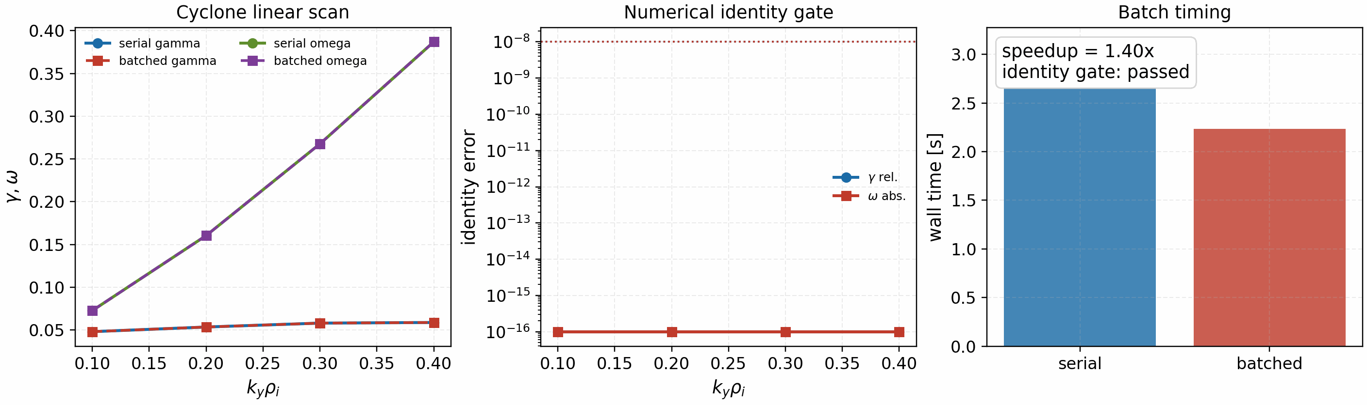
It is regenerated with:

python tools/artifacts/generate_parallel_identity_gate.py ky-scan

This gate runs the same linear solver serially and with fixed-shape k_y batching, checks gamma and omega numerical identity, and reports observed speedup as an engineering metric. The gate intentionally does not claim nonlinear domain scaling; that remains a separate communication and FFT-decomposition problem.

The complementary logical-CPU gate exercises the public RuntimeParallelConfig and batch_map interface on a structured JAX pytree output. It is not a gyrokinetic physics validation; it verifies that the parallel API preserves serial numerical identity for independent scan/UQ-style workloads before those workloads are connected to heavier solver paths.

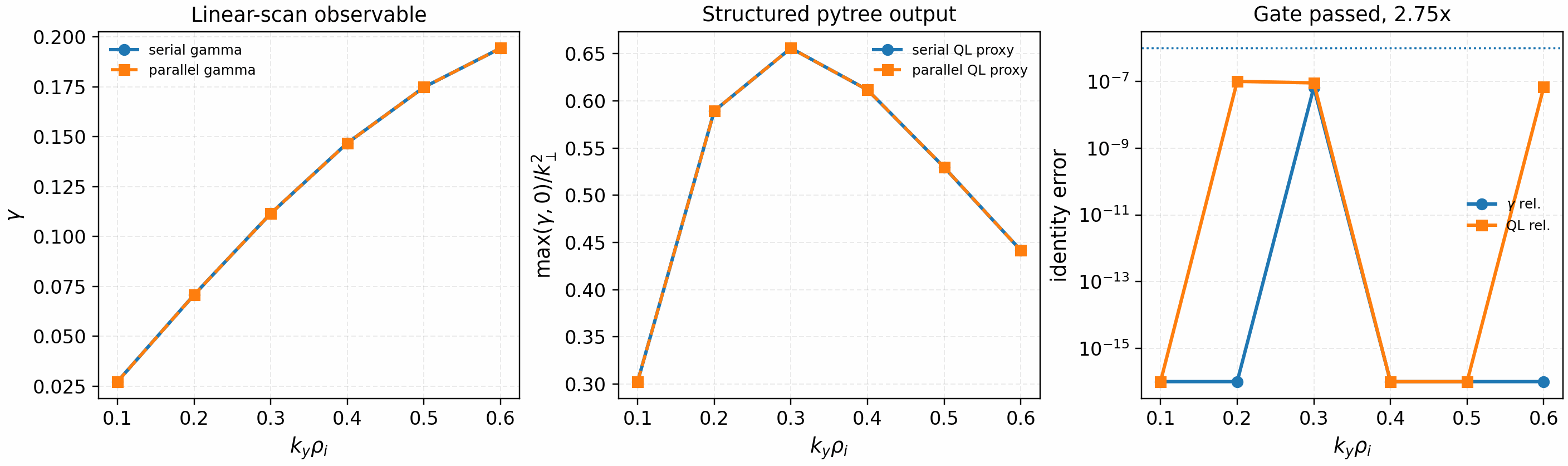
It is regenerated with:

python tools/artifacts/generate_parallel_identity_gate.py logical-cpu --logical-devices 2

The tracked artifact used two logical CPU devices and passed the identity gate: max_gamma_rel_error=6.7e-8, max_ql_rel_error=1.1e-7, and max_omega_abs_error=0. The observed timing is retained as engineering metadata only; a speedup claim requires a solver-backed workload and fresh CPU/GPU profiler artifacts.

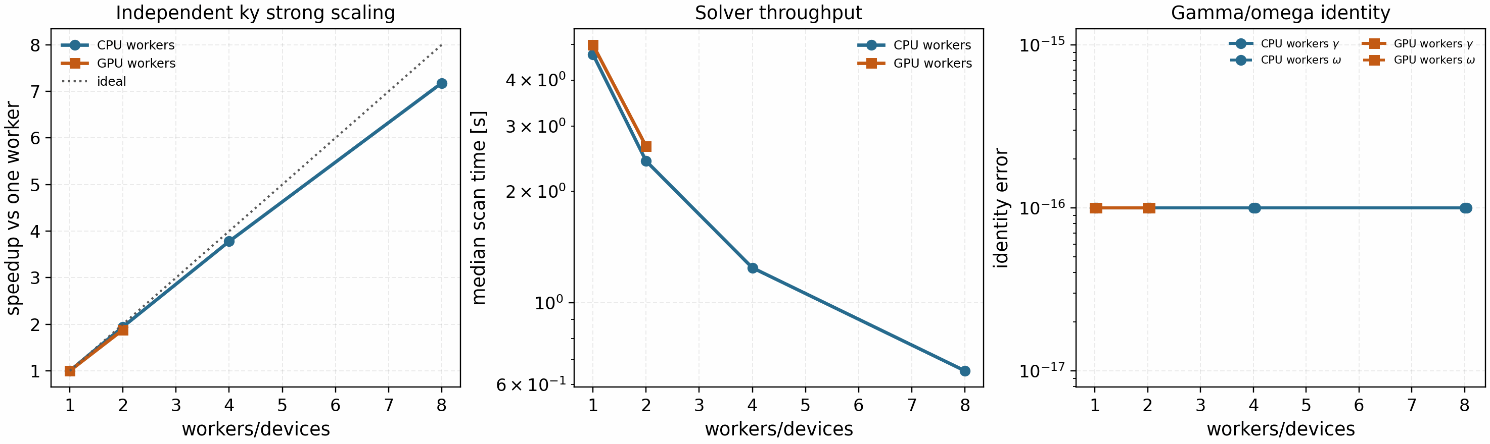
The solver-backed strong-scaling artifact now exercises that production policy on a larger real Cyclone linear scan with 64 independent k_y values, Ny=128, Nz=96, Nl=4, Nm=8, and 240 RK2 steps per mode. Each worker performs one warmup scan before the timed repeats, and every multi-worker result is compared against the one-worker reference for gamma and omega identity:

It is regenerated with:

KY=$(python -c "print(','.join(f'{0.04 + 0.0125*i:.3f}' for i in range(64)))")

python tools/profiling/profile_parallel_workloads.py independent-ky \
  --backend cpu --devices 1,2,4,8 \
  --ky "$KY" \
  --ny 128 --nz 96 --nl 4 --nm 8 --steps 240 \
  --out-prefix docs/_static/independent_ky_scan_scaling_cpu_large

python tools/profiling/profile_parallel_workloads.py independent-ky \
  --backend gpu --devices 1,2 \
  --ky "$KY" \
  --ny 128 --nz 96 --nl 4 --nm 8 --steps 240 \
  --out-prefix docs/_static/independent_ky_scan_scaling_gpu_large

python tools/artifacts/plot_scaling_panels.py independent-ky

The May 12, 2026 refresh passes the identity gate with zero reported gamma/omega mismatch. CPU process scaling reaches 1.94x on two workers, 3.78x on four workers, and 7.18x on eight workers. The two-GPU RTX A4000 run reaches 1.88x with about 94% parallel efficiency. This is the current recommended production parallelization path for linear scans, quasilinear studies, and UQ ensembles: it has much better scaling behavior than whole-state nonlinear sharding because communication is restricted to post-run result aggregation. Sensitivity sweeps are covered by the same ordering/provenance utilities, but need their own scaling artifact before any speedup claim is promoted.

The release closure status is machine-readable and separates production claims from diagnostic decomposition work:

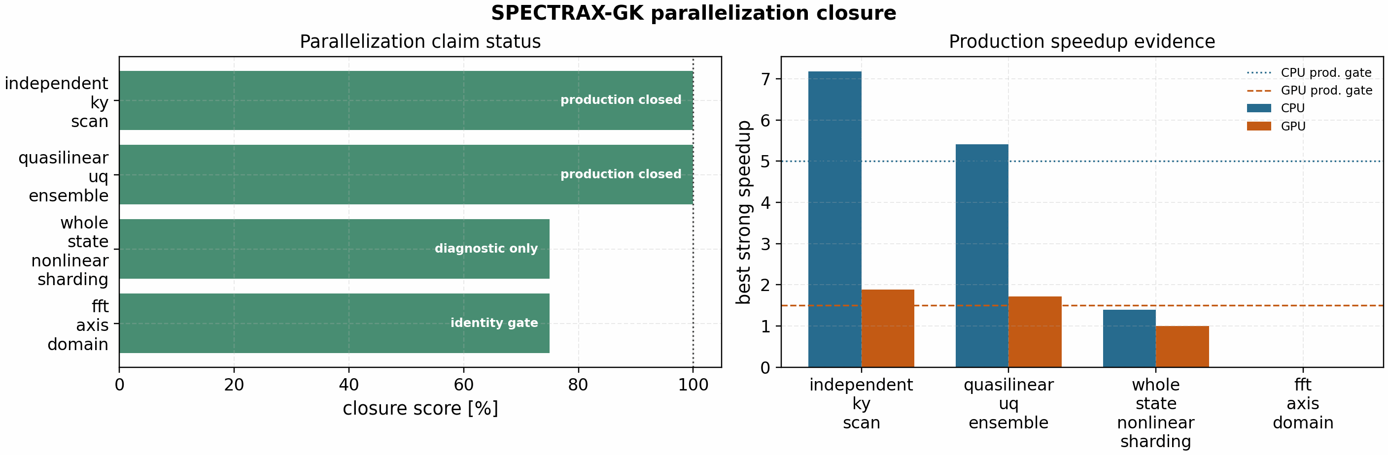
The tracked docs/_static/parallelization_completion_status.json reports production_completion_percent = 100 for independent k_y scans and quasilinear/UQ ensembles. The same artifact keeps whole-state nonlinear sharding and FFT-axis decomposition at diagnostic status until runtime distributed communication, conservation, transport-window, and profiler-backed speedup gates are closed.

The nonlinear state-domain prototype now has a stronger diagnostic gate in docs/_static/nonlinear_domain_parallel_identity_gate.json. In addition to the one-step serial-vs-halo-decomposed state check, the embedded nonlinear_domain_transport_window_identity report advances a short fixed-step window and compares boundary identity plus mass, free-energy-proxy, and boundary-flux-proxy traces. Those trace drifts are agreement metadata for the diagnostic local stencil only. They do not validate production conservation, distributed FFT routing, field solves, benchmark transport windows, or any speedup claim.

The tracked spectral-domain routing profile adds a work model for the current global-reconstruction diagnostic route. It passes serial-vs-routed identity, but the four-tile profile reports communication/owned-work ratio 6.375, a parallel-efficiency ceiling 0.136, and measured warm timing 0.94x. This is negative performance evidence for the current route and points to the actual implementation target: avoid global state/bracket reconstruction by using a communication-aware distributed FFT and fused nonlinear-bracket route.

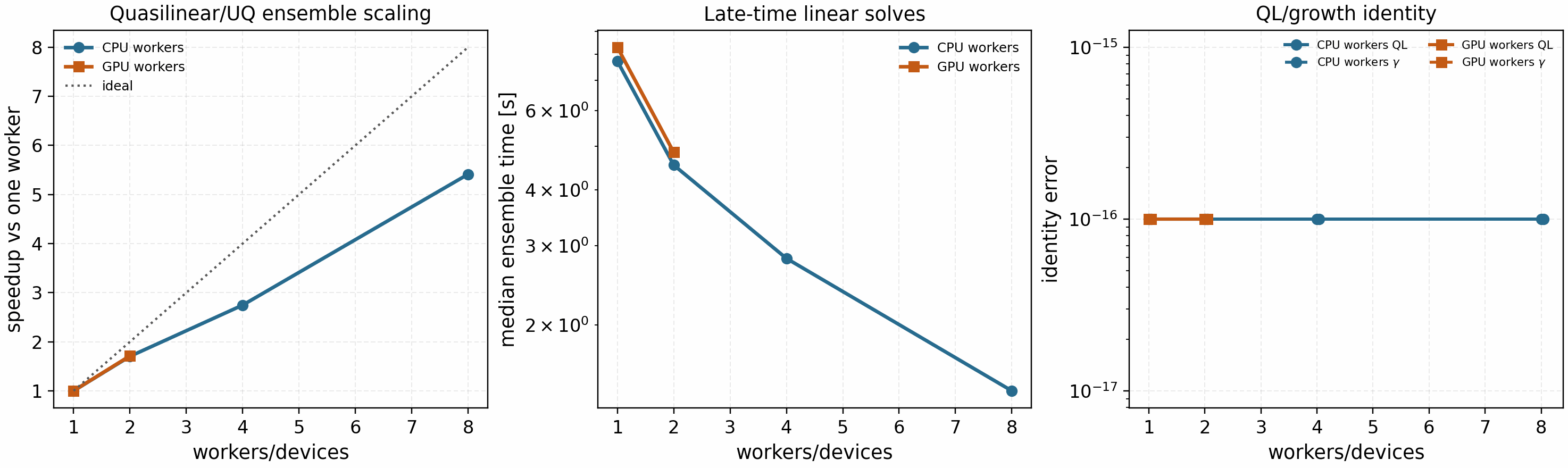
The same independent-worker policy is also gated on a quasilinear/UQ-style ensemble: six late-time Cyclone ITG gradient samples, five k_y values per sample, Ny=96, Nz=64, Nl=3, Nm=6, and 2000 RK2 steps per mode. Each worker computes real late-time linear growth/frequency fits and a reduced mixing-length feature observable. The observable is useful for parallelization and UQ plumbing, but it is not promoted as an absolute nonlinear heat-flux predictor.

It is regenerated with:

python tools/profiling/profile_parallel_workloads.py quasilinear-uq \
  --backend cpu --devices 1,2,4,8 \
  --out-prefix docs/_static/quasilinear_uq_ensemble_scaling_cpu_large

python tools/profiling/profile_parallel_workloads.py quasilinear-uq \
  --backend gpu --devices 1,2 \
  --out-prefix docs/_static/quasilinear_uq_ensemble_scaling_gpu_large

python tools/artifacts/plot_quasilinear_diagnostics.py uq-ensemble-scaling

The May 10, 2026 office sweep passes the serial identity gate for both the reduced quasilinear proxy and gamma. The CPU run reaches 1.70x on two workers, 2.75x on four workers, and 5.41x on eight requested workers using six actual ensemble chunks. The two-GPU RTX A4000 run reaches 1.71x with about 86% parallel efficiency. This closes the release engineering gate for quasilinear calibration grids, finite-difference checks, sensitivity sweeps, and UQ ensembles that can be decomposed into independent solver calls.

Nonlinear-decomposition promotion follows the same conservative rule. gkx.build_velocity_sharding_plan records a species-first, Hermite-second velocity-space layout, including which axes need Hermite ghost exchange and which axes need field-solve reductions and broadcasts. Periodic and linked 2 species x 2 Hermite electrostatic operator routes now pass identity gates, but their communication evidence does not establish nonlinear transport speedup. Mixed electromagnetic integration and profiler-backed four-device evidence remain required before broadening that claim.

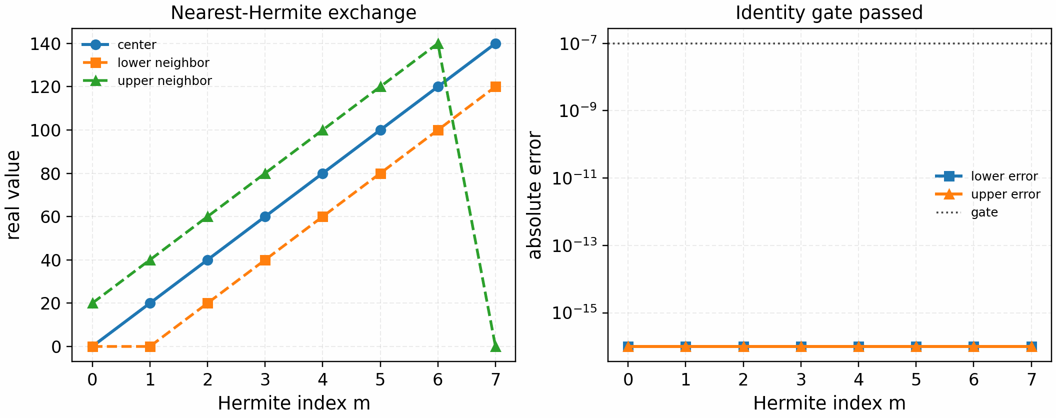
The first concrete communication-kernel gate is the Hermite ghost exchange. It uses jax.shard_map to exchange nearest-neighbor Hermite moments across a two-device logical CPU mesh and compares the result against the full-array reference shift with zero physical boundaries:

It is regenerated with:

python tools/artifacts/generate_velocity_parallel_gates.py hermite-exchange --logical-devices 2

The tracked artifact passes with zero reported lower/upper neighbor error. It only validates the communication primitive. Promoting nonlinear velocity-space decomposition beyond diagnostic evidence still needs field-reduction/broadcast gates, streaming-operator identity gates, full-RHS identity gates, and profiler artifacts before any speedup claim.

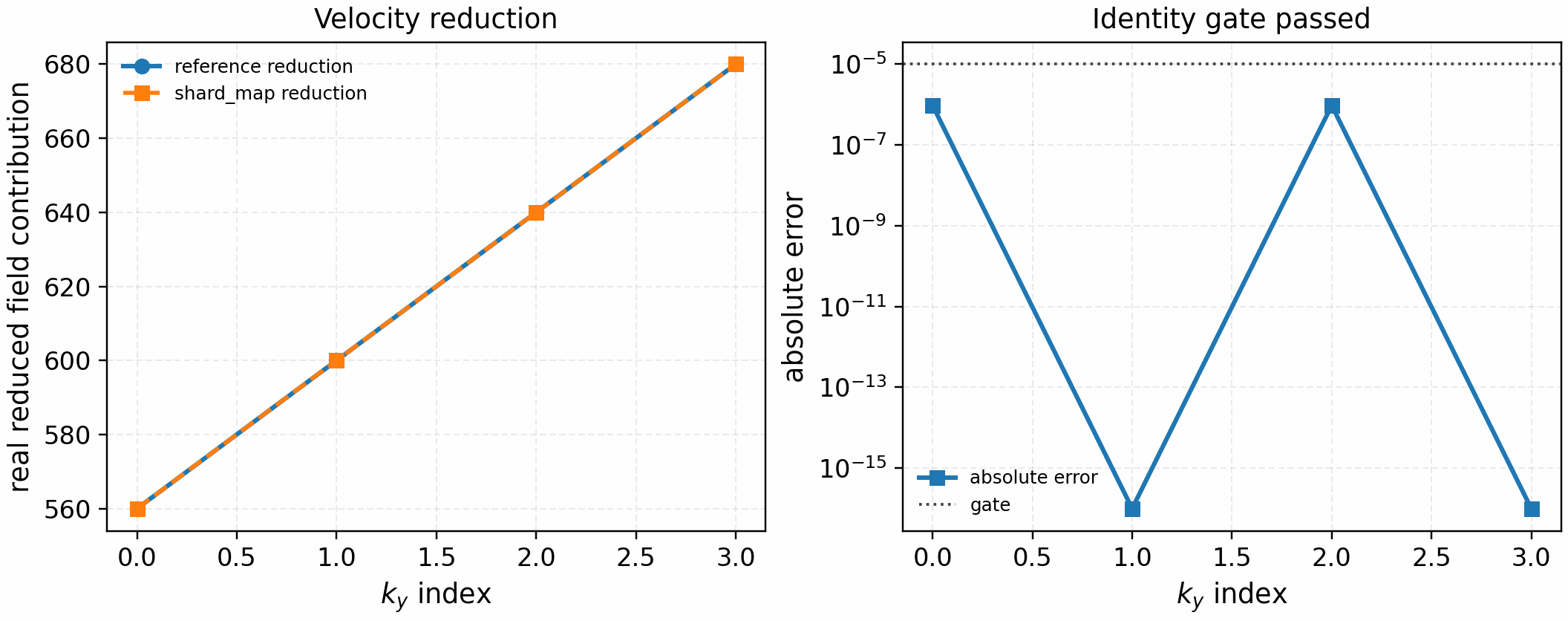
The matching velocity-space field-reduction gate validates the second required communication primitive. It reduces the Hermite-sharded local contributions with lax.psum and compares against the full-array reference sum:

It is regenerated with:

python tools/artifacts/generate_velocity_parallel_gates.py field-reduce --logical-devices 2

The tracked artifact passes with max_abs_error=3.9e-6 under an absolute tolerance of 1e-5. This tolerance reflects expected float32 roundoff from a different reduction tree; it is not a physics tolerance. The next gate must combine Hermite exchange and field reduction with the actual streaming coefficients.

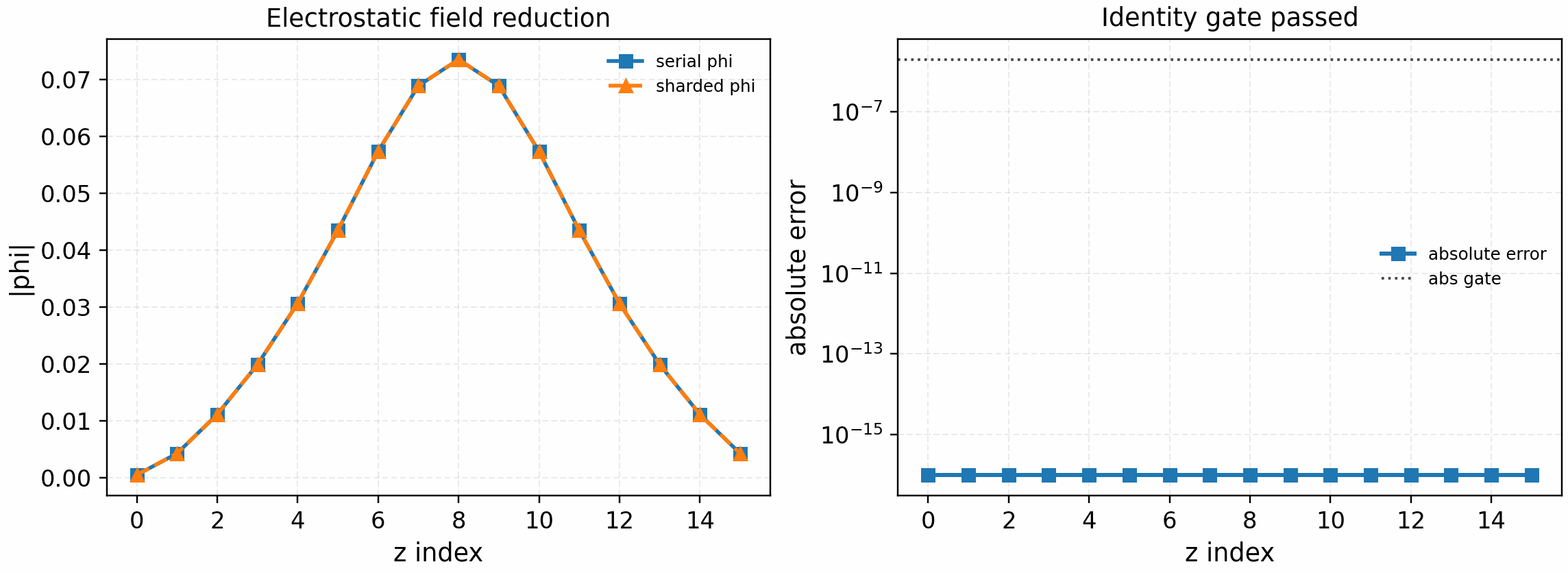
The electrostatic field-reduction gate applies the same lax.psum pattern to the actual m=0 density moment used by quasineutrality and compares the resulting phi against the production field solve:

It is regenerated with:

python tools/artifacts/generate_electrostatic_parallel_gates.py field-reduce --logical-devices 2

The tracked artifact passes exactly on the current single-species periodic gate with phi_norm=1.68e-1 and zero reported absolute/relative error. This is the first true sharded field-reduction solve gate; multi-species, linked-boundary, electromagnetic, and nonlinear field solves remain separate gates.

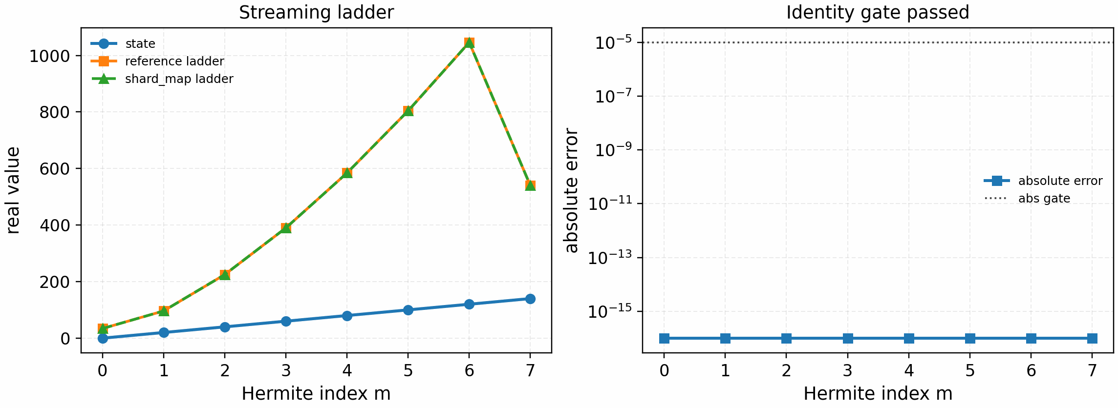
That coefficient gate is now tracked separately. It applies the sqrt(m+1) upper-neighbor and sqrt(m) lower-neighbor Hermite streaming ladder on top of the shard-map exchange and records the paired field-reduction error:

It is regenerated with:

python tools/artifacts/generate_velocity_parallel_gates.py hermite-ladder --logical-devices 2

The tracked artifact passes with zero ladder error and records an accompanying Hermite field-reduction error of 1.9e-6. This closes the communication and coefficient layer for a one-dimensional Hermite mesh. The next step is an opt-in linear streaming microkernel that includes the actual parallel derivative contract.

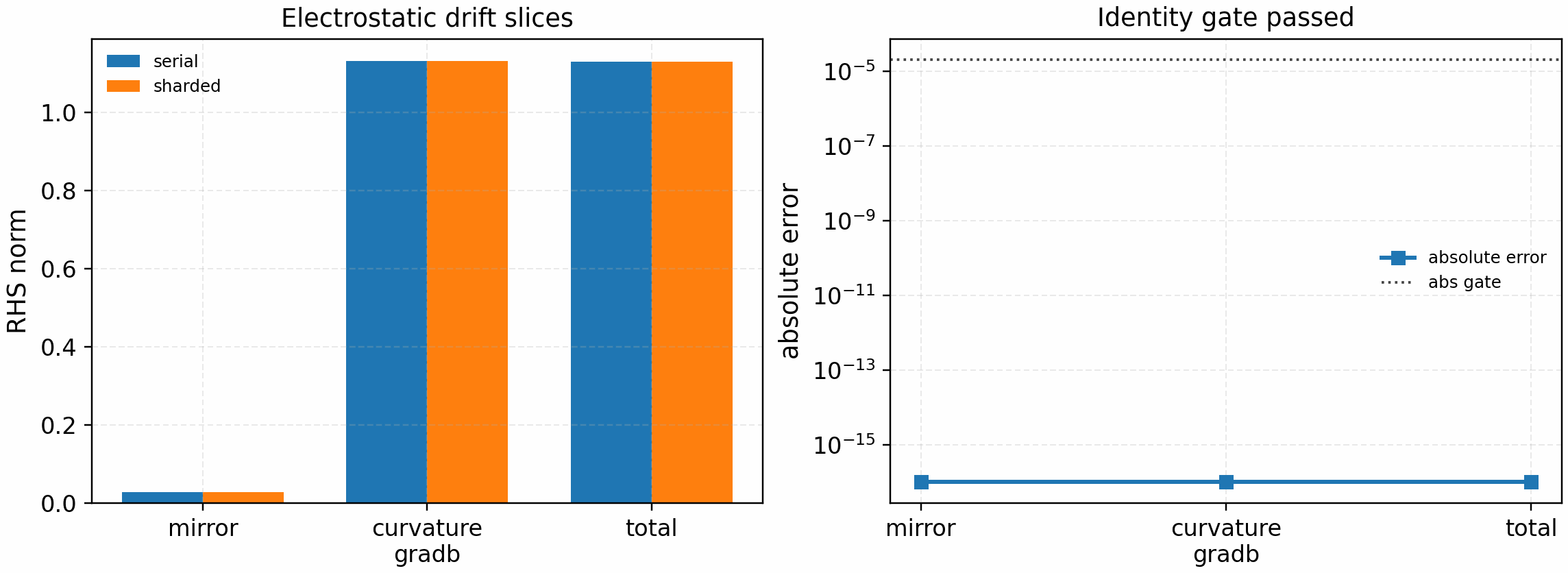
The electrostatic drift-slice gate then uses offset-1 and offset-2 Hermite exchanges for mirror and curvature terms, together with the electrostatic field-reduction gate:

It is regenerated with:

python tools/artifacts/generate_electrostatic_parallel_gates.py drift --logical-devices 2

The tracked artifact passes with phi_norm=1.21e-1 and zero reported absolute/relative error for the mirror, curvature/grad-B, and combined drift slices. This is a single-species periodic electrostatic identity gate, not a full-RHS, linked-boundary, electromagnetic, or nonlinear performance claim. The gated slices are available together through gkx.linear_rhs_parallel_cached with RuntimeParallelConfig(strategy="velocity", axis="hermite", backend="electrostatic_linear_slices").

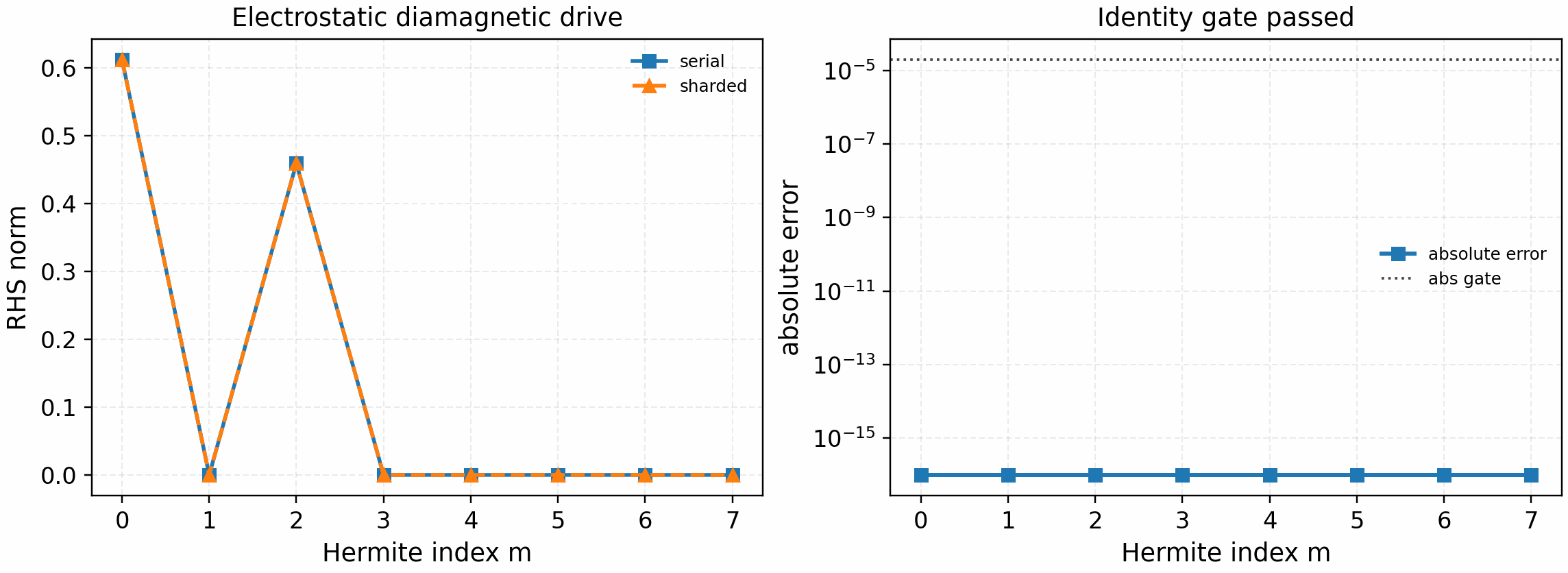
The electrostatic diamagnetic-drive gate validates the remaining local electrostatic drive slice. It uses the Hermite-sharded electrostatic field reduction, then applies the local m=0 and m=2 density/temperature gradient masks on each Hermite shard:

It is regenerated with:

python tools/artifacts/generate_electrostatic_parallel_gates.py diamagnetic --logical-devices 2

The tracked artifact passes with phi_norm=1.68e-1 and zero reported absolute/relative error against the production diamagnetic-only linear RHS. The opt-in backend="electrostatic_linear_slices" route now combines streaming, mirror, curvature, grad-B, and diamagnetic slices. It still rejects collision, electromagnetic, linked-boundary, multi-species, and nonlinear terms until each path has its own identity gate.

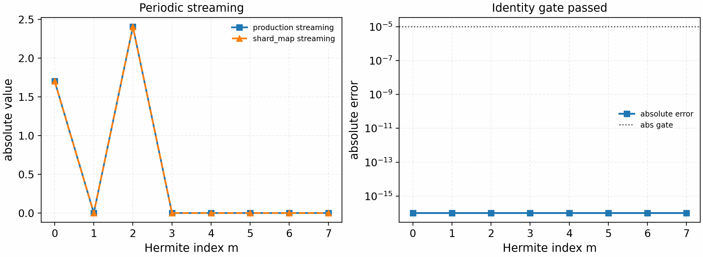
The periodic linear-streaming microkernel gate then adds the spectral parallel derivative along the field-line direction and compares the resulting shard_map path directly against the production gkx.operators.linear.streaming.streaming_ladder_term:

It is regenerated with:

python tools/artifacts/generate_velocity_parallel_gates.py periodic-streaming --logical-devices 2

The tracked artifact passes with zero reported absolute and relative error. This is still a linear streaming microkernel gate, not a full linear RHS or nonlinear performance claim.

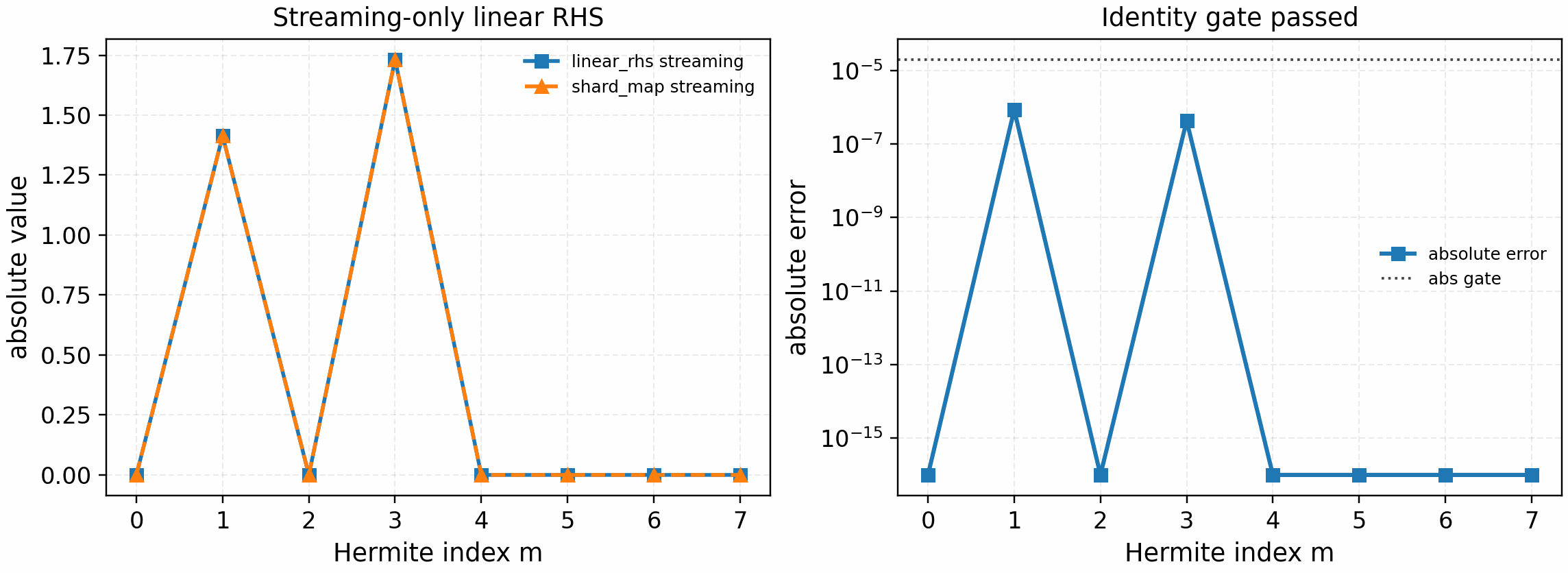
The next release gate exercises the same periodic streaming path through the production linear_rhs_cached call graph. The artifact disables all non-streaming terms, keeps electromagnetic channels off, and uses non-density Hermite moments so that the electrostatic field solve is exactly zero:

It is regenerated with:

python tools/artifacts/generate_linear_rhs_parallel_gates.py streaming --logical-devices 2

The tracked artifact passes with max_abs_error=9.7e-7, max_rel_error=5.6e-7, and phi_norm=0. This closes a streaming-only linear-RHS identity gate. It deliberately does not claim full-RHS, nonlinear, or production speedup parity; those remain separate gates with additional field-solve, drive, collision, bracket, and profiler coverage.

For code-level experiments the same route is available through gkx.linear_rhs_parallel_cached with RuntimeParallelConfig(strategy="velocity", axis="hermite", backend="streaming_only"). The helper rejects any non-streaming term weights so this remains a disabled-by-default diagnostic path rather than a hidden solver change.

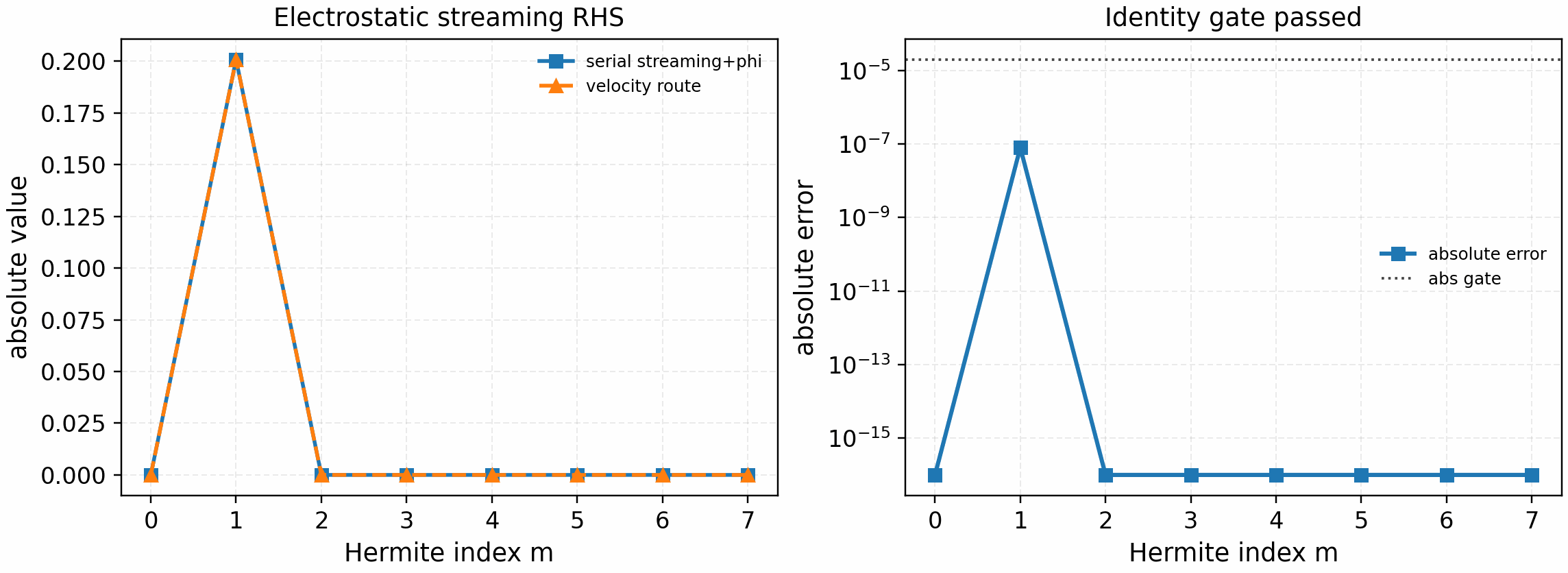
The follow-on electrostatic streaming gate keeps the term weights identical but initializes an m=0 density perturbation so that the production electrostatic field solve produces nonzero phi. It then compares linear_rhs_cached against the explicit backend="streaming_electrostatic" route:

It is regenerated with:

python tools/artifacts/generate_linear_rhs_parallel_gates.py streaming-electrostatic --logical-devices 2

The tracked artifact passes with phi_norm=1.34e-1, max_phi_abs_error=1.9e-9, max_abs_error=1.4e-7, and max_rel_error=4.1e-7. The field solve uses the single-species Hermite-sharded electrostatic reduction gate above; this validates the field-reduction-to-streaming call graph before the drift, diamagnetic-drive, and nonlinear paths are introduced.

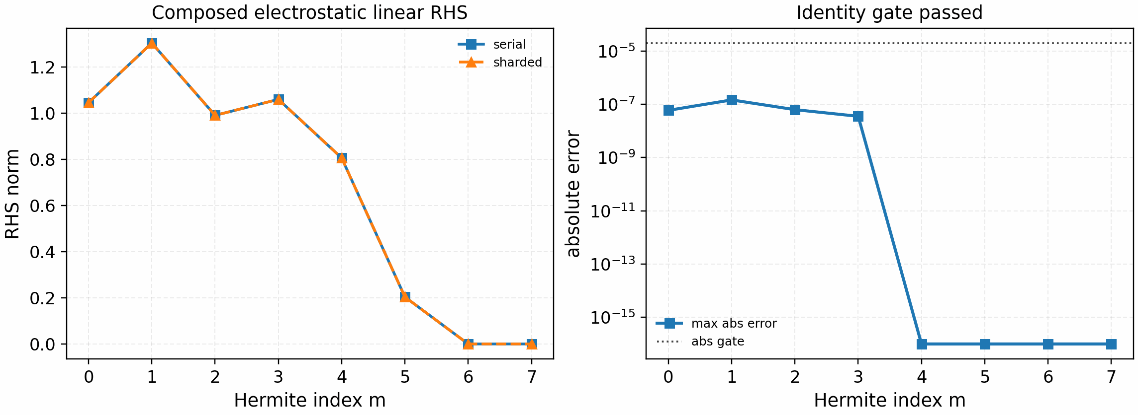
The current composed electrostatic linear-RHS gate then exercises the opt-in backend="electrostatic_linear_slices" route against the serial production RHS with streaming, mirror, curvature, grad-B, and diamagnetic drive enabled:

It is regenerated with:

python tools/artifacts/generate_linear_rhs_parallel_gates.py electrostatic-slices --logical-devices 2

The tracked artifact passes with phi_norm=1.68e-1, max_abs_error=1.5e-7, max_rel_error=3.7e-7, and zero reported electrostatic-potential error. This is the current single-species periodic electrostatic linear-RHS identity gate for velocity-space parallelization. It is not a linked-boundary, collision, electromagnetic, nonlinear, or speedup claim.

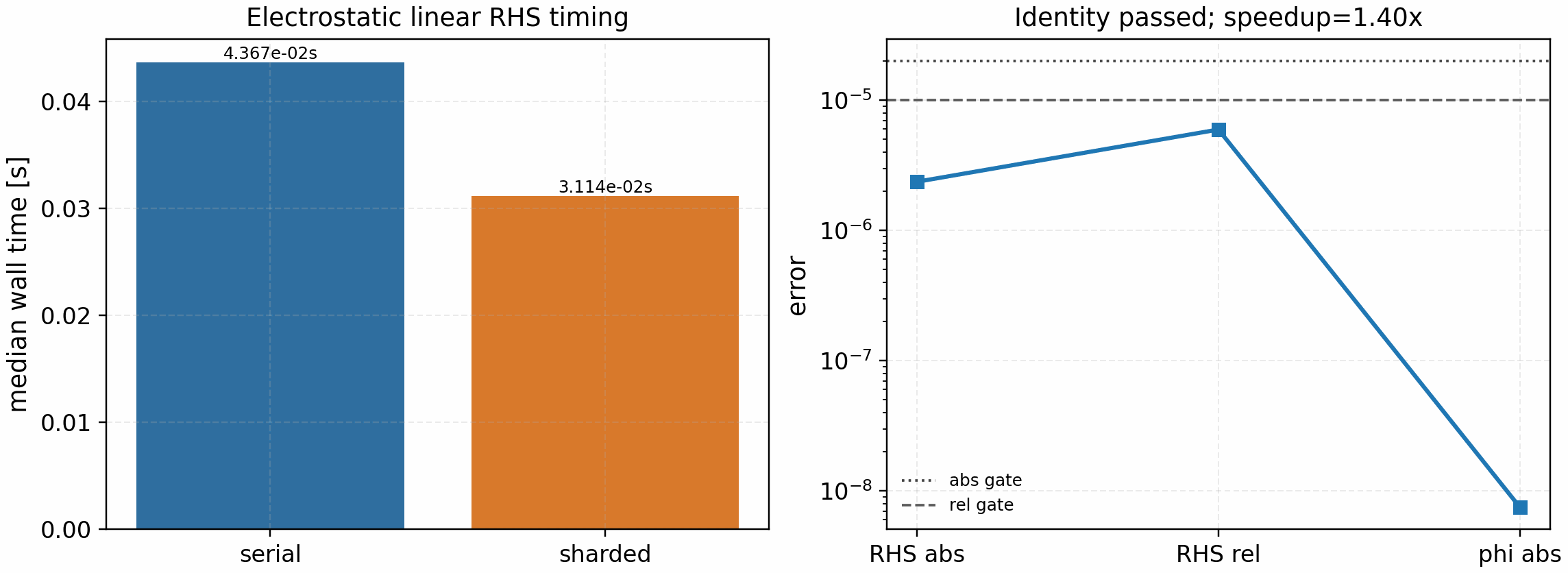
The matching engineering profile intentionally stays separate from the identity gate:

It is regenerated with:

python tools/profiling/profile_linear_rhs_parallel_slices.py \
  --logical-devices 8 --nl 4 --nm 128 --ny 32 --nz 128 --rtol 1e-5

The tracked CPU artifact uses a Hermite-heavy workload and keeps the sharded route within a float32 reduction-order engineering tolerance: max_abs_error=2.4e-6, max_rel_error=6.0e-6, and max_phi_abs_error=7.5e-9. The warm timings are serial_median_s=4.37e-2, sharded_median_s=3.11e-2, and speedup=1.40x on eight logical CPU devices. This remains an engineering profile rather than a publication speedup claim; the stricter small-grid identity gate above is the release correctness gate.

A compact CPU sweep maps the same opt-in route across Hermite resolution and logical device count:

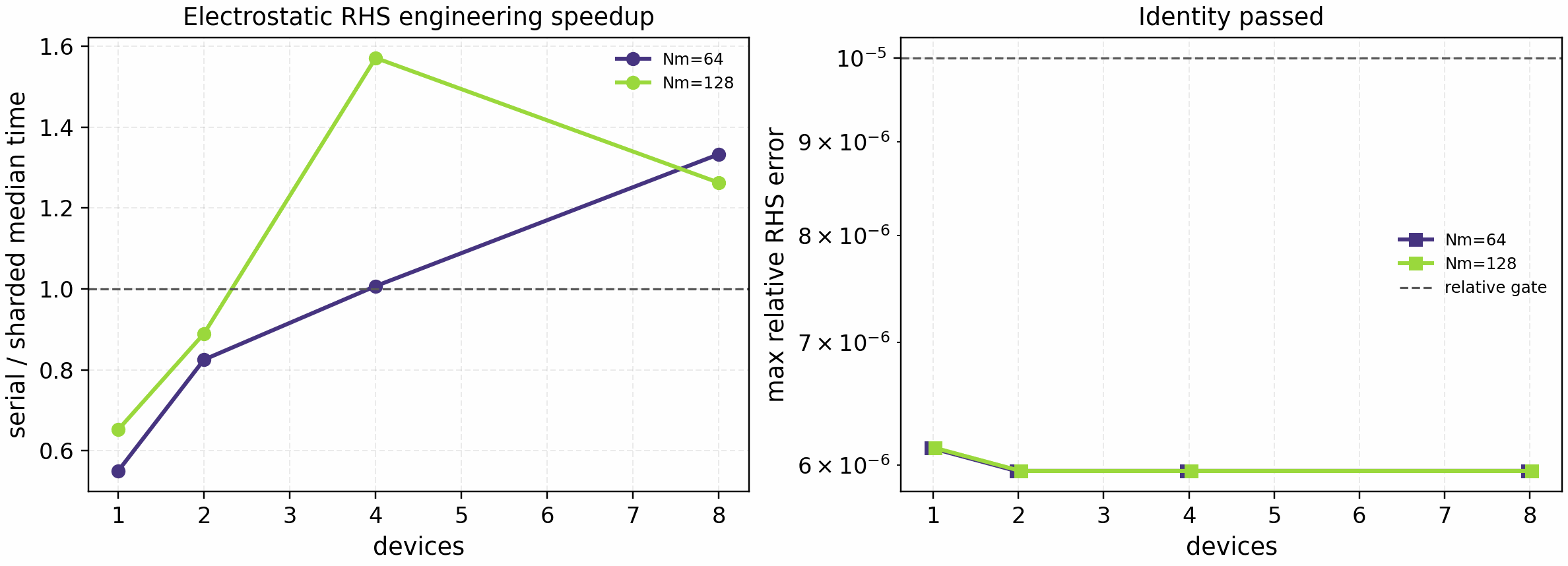
It is regenerated with:

python tools/profiling/profile_linear_rhs_parallel_slices.py sweep \
  --platform cpu --devices 1,2,4,8 --nms 64,128 \
  --nl 4 --ny 32 --nz 128 --rtol 1e-5

The tracked sweep passes identity for all points. It shows the current Hermite-sharded electrostatic route is overhead-limited at one and two logical CPU devices, becomes competitive near four devices, and reaches the best bounded engineering point of 1.57x at Nm=128 on four logical CPU devices. This figure is a regime map for development, not a broad scaling claim. The machine-readable release contract is docs/_static/linear_rhs_parallel_slices_sweep.json with CSV/PNG/PDF companions.

The same profiler can target GPUs on the office node:

PYTHONPATH=/tmp/gkx-profile/src python3 \
  tools/profiling/profile_linear_rhs_parallel_slices.py \
  --platform gpu --logical-devices 2 \
  --nl 4 --nm 64 --ny 32 --nz 128 --rtol 1e-5 \
  --out-prefix docs/_static/linear_rhs_parallel_slices_profile_gpu

The tracked two-RTX-A4000 artifact passes the engineering identity check (max_abs_error=1.9e-6, max_rel_error=4.7e-6), but it is much slower than the single-GPU serial JIT path (speedup=0.03x). This keeps the GPU Hermite-sharding lane open: do not claim GPU speedup until the communication layout is redesigned or a larger production workload shows a real gain.

The species-first kinetic-electron route uses the same profiler with --axis species. The tracked two-A4000, 2x8x32x128x1x128 state passes the host-reduced identity gate with max_rel_error=5.26e-8 and max_phi_abs_error=6.59e-10. Its warm medians are 8.21 ms on one GPU and 7.11 ms on two GPUs, a scoped 1.16x speedup. The smaller 2x4x16x64x1x64 engineering probe was slower on two GPUs, so this is a large-workload crossover result, not a broad strong-scaling claim. The evidence is retained in docs/_static/linear_rhs_species_profile_gpu.json and is regenerated with:

python tools/profiling/profile_linear_rhs_parallel_slices.py \
  --axis species --platform gpu --logical-devices 2 \
  --nl 8 --nm 32 --ny 128 --nz 128 --warmups 2 --repeats 10 \
  --out-prefix /tmp/linear_rhs_species_profile_gpu

The same profiler can include a full fixed-step integration gate with --integration-steps. The tracked two-logical-CPU artifact uses 100 Euler steps on a 2x4x16x64x1x64 state. The enclosing pmap agrees exactly with serial state and field histories. After removing replicated field-history output and aligning sampled diagnostics with the serial policy, the refreshed artifact reaches 3.41x for isolated RHS calls and 0.96x for the complete 100-step trajectory. It therefore remains a correctness and crossover artifact, not an end-to-end speedup claim. It is stored in docs/_static/linear_rhs_species_profile_cpu.json and regenerated with:

python tools/profiling/profile_linear_rhs_parallel_slices.py \
  --axis species --platform cpu --logical-devices 2 \
  --nl 4 --nm 16 --ny 64 --nz 64 --warmups 2 --repeats 5 \
  --integration-steps 100 --integration-repeats 5 \
  --integration-sample-stride 1 \
  --out-prefix /tmp/linear_rhs_species_profile_cpu

An uncontended two-GPU integration artifact is still required before promoting an end-to-end species-parallel speedup; concurrent office workloads invalidated the available timing samples but not their host-reduced identity checks.

The mixed species–Hermite profile uses four logical CPU devices. On the periodic collision-free electrostatic 2x4x16x64x1x64 workload, the (species,m)=(2,2) mesh matches the serial RHS to 5.6e-8 relative and reaches a scoped 3.11x warm-RHS speedup. It applies streaming, mirror, curvature, grad-\(B\), and diamagnetic terms. The same artifact advances 100 Euler steps with exact state/field histories but only 0.97x end-to-end throughput, so no integration-speedup claim is made. This is not evidence for general strong scaling, GPUs, linked boundaries, or collisions. The machine-readable evidence is docs/_static/linear_rhs_species_hermite_profile_cpu.json and is regenerated with:

python tools/profiling/profile_linear_rhs_parallel_slices.py \
  --axis species_hermite --platform cpu --logical-devices 4 \
  --nl 4 --nm 16 --ny 64 --nz 64 --warmups 2 --repeats 7 \
  --integration-steps 100 --integration-repeats 5 \
  --integration-dt 1e-7 --integration-sample-stride 1 \
  --out-prefix /tmp/linear_rhs_species_hermite_profile_cpu

Fixed-step nonlinear state sharding

The fixed-step nonlinear runner now has the same full-state sharding contract as the linear path for release-gated state axes. Set TimeConfig.state_sharding = "auto" (or a concrete axis such as "ky" or "kx") with use_diffrax = false to route through gkx.integrate_nonlinear_sharded. The implementation uses a pjit scan and preserves the serial Runge-Kutta update; it is therefore an identity-gated state-sharding primitive, not a halo-exchange FFT domain decomposition claim. Sharding the z FFT axis is deliberately not exposed as a release-gated nonlinear runtime path because the current JAX/XLA FFT layout does not pass the multi-device identity gate.

The profiler/identity artifact is generated with:

python tools/profiling/profile_nonlinear_sharding.py \
  --sharding auto --sharding-options auto,kx \
  --out-json docs/_static/nonlinear_sharding_profile.json

The JSON records device count, requested sharding axis, warm serial/sharded timings, profiler-trace status, final-state errors, final-field/RHS diagnostic errors, and the fastest identity-preserving candidate among the requested state-axis options. Refreshed profiler outputs also carry a versioned source contract with the exact command, command argv, source artifact, backend, device count, sharding axis, warmup/repeat policy, and Python/JAX/NumPy/GKX versions. The fast parallel artifact checker validates that contract whenever it is present; older checked-in diagnostic profiles remain scoped until they are refreshed with the same metadata. The local checked-in artifact is deliberately small and only establishes the control-flow and single-device identity gate. Its constant ky=0, kx=0 state has a zero nonlinear bracket and is superseded for physical identity decisions. The older two-GPU office artifact at docs/_static/nonlinear_sharding_profile_office_gpu.json is likewise a tiny (4,6,8,4,16) smoke test: it records zero state error but no speedup. It must not be generalized to a transport grid. The matched benchmark-grid artifact, docs/_static/nonlinear_sharding_profile_office_gpu_benchmark_grid.json, uses (4,8,64,192,24) and 20 fixed RK2 steps. Active kx sharding is slower than serial (0.211x) and fails trajectory identity (max_abs_state_error=20.0). The final RHS also differs by max_abs_rhs_error=1279.39; a zero potential difference alone is not a sufficient diagnostic identity gate. Therefore whole-state nonlinear sharding is blocked from production routing and runtime claims. The next implementation must change the decomposition, not relax this gate.

The clean-revision physical refresh is docs/_static/nonlinear_sharding_profile_office_gpu_physical.json. It uses three interacting spectral perturbations on a (4,8,32,32,64) state for 100 RK2 steps and records a nonzero initial nonlinear RHS. On two RTX A4000 GPUs, serial execution takes 3.77 s, while ky and kx whole-state placement take 9.19 s and 7.22 s; both fail final-state and RHS identity. This artifact controls the current conclusion and prevents zero-bracket smoke tests from being promoted as nonlinear decomposition evidence.

For final-state-only optimization or profiling, the explicit scan accepts return_fields=False. This avoids one post-step RHS evaluation that exists only to materialize final field history. On the same office GPU and (4,8,64,192,24) workload, a controlled same-process A/B measurement reduced the median warm 20-step time by about 5–6%. This is a narrowly scoped engineering result, not a refreshed end-to-end application speed claim.

The fixed-step profiler also exposed a compilation-cache defect: both serial and sharded integration wrappers created new static Python closures on every call, so nominal warm repeats could compile again. The integration API now passes cache and parameter pytrees dynamically, keeps only mathematical switches static, memoizes the small grid projector, and reuses a compiled sharded runner. On the local (2,4,8,8,8) two-step smoke workload, three post-warmup serial calls take 0.78--0.90 ms and the diagnostic sharded wrapper takes 0.99--1.07 ms with exact state identity; before the fix the same sharded wrapper took about 0.41 s per repeat. The refreshed office artifact at clean commit 91c0c2a7 records a serial median of 0.893 s and a diagnostic two-GPU median of 4.22 s for 20 RK2 steps. The prior serial artifact reported 15.37 s because nominal warm repeats recompiled. This is a substantial single-GPU execution fix, but it is not a multi-device speedup: the decomposition remains both slower and numerically invalid.

The end-to-end runtime profiler now blocks every returned JAX leaf before stopping its timer and validates that its default input exists. It also accepts --repeats and reports each completed warm timing. On the shipped Cyclone 64x64x24 CPU input, a bounded 20-step run at sample_stride=diagnostics_stride=10 takes 6.05 s warm after a 12.84 s cold pass. This is a profiler baseline, not a publication runtime row. The matched office A4000 run takes 9.78 s warm with resolved spectra and 8.69 s with compact scalar diagnostics. The compact route therefore saves about 11% on this moderate GPU workload, while the matched local CPU improvement is about 3%. A final-state-only fixed-step GPU integration takes 0.263 s on the same grid, showing that setup, synchronization, and diagnostic materialization dominate this short end-to-end workload. These are profiling results, not universal GPU speedup claims. Artifact-producing runs can request the compact route explicitly with [output] resolved_diagnostics = false when mode-resolved spectra are not needed.

Repeated Python simulations should prepare the explicit nonlinear diagnostic scan once instead of rebuilding its closure for every objective or ensemble evaluation:

from gkx.solvers.nonlinear.diagnostic_integration import prepare_nonlinear_explicit_diagnostics

simulation = prepare_nonlinear_explicit_diagnostics(
    initial_state, grid, geometry, parameters,
    dt=0.02, steps=400, resolved_diagnostics=False,
)
final_state, diagnostics, time_step, fields = simulation.run()

simulation.run(new_initial_state) reuses the compiled scan for states with the same shape and dtype. Method, grid layout, and diagnostic schema are fixed by this prepared contract. Fixed-step parameter studies may pass a matched rebuilt cache and parameter PyTree with simulation.run(cache=new_cache, params=new_params); supplying only one is rejected because gyroaverages, drifts, and collision arrays would be inconsistent.

For sensitivity calculations, simulation.run_arrays(new_initial_state) returns only JAX pytrees and skips host-side diagnostic finalization. Reverse mode therefore differentiates through the explicit time loop with respect to the initial state. On fixed-step runs it also differentiates through matched dynamic (geometry, cache, params) inputs; the cache must be rebuilt from the same traced geometry and parameters before the call. A physical nonzonal-mode gate scales curvature and grad-B profiles, propagates the changed geometry through cache construction and three RK2 steps, and matches a centered finite difference derivative. Grid shape, geometry sampling layout, method, and output schema remain static. The current field-solve custom VJP supports this reverse-mode path but not a forward-mode JVP through the full scan. Adaptive prepared execution remains available for ordinary state runs, while traced geometry/cache/parameter overrides fail closed until adaptive-controller derivative policy gates are implemented.

On the shipped 64x64x24 Cyclone setup, a three-call CPU compile-log gate records exactly one jit(run_raw) compilation. The first two-step call takes 3.25 s including compilation; repeated calls take 0.297 s and 0.290 s. Rebuilding the runtime closure took 2.27--2.29 s for the same nominal warm calls. This is a repeated Python-call improvement for fixed geometry/model policy, not an end-to-end executable or long-run throughput claim.

The current controlled prepared profiles are tracked as prepared_nonlinear_runtime_cpu_profile.json and prepared_nonlinear_runtime_gpu_profile.json. Both use commit d3f3aef8, Python 3.10.12, JAX 0.6.2, NumPy 2.2.4, adaptive RK3, 200 steps, diagnostic stride 10, and compact scalar diagnostics on the same office node. The CPU warm run takes 109.275 s and one RTX A4000 takes 9.338 s, a measured 11.70x device-throughput ratio after separate compilation. This is not an end-to-end executable or multi-GPU scaling claim. The final-state norm is identical at recorded precision; timestep, potential, and heat-flux norms agree within 3.8e-6 relative. The profiler and artifact gate now require these numerical fingerprints, matched software/configuration, and at least a 5x ratio before the row can remain promoted.

Matched resolved-diagnostic profiles use the same 200-step trajectory and produce exactly the same recorded final-state, potential, heat-flux, and timestep norms. On CPU, retaining mode-resolved histories adds 0.62% warm time and 1.18% peak host RSS. On the A4000, three-repeat medians show 2.36% warm-time overhead, 2.78% peak device-memory overhead, 5.38% additional live device allocation, and 2.61% peak host-RSS overhead. The artifact gate permits at most 25% runtime and 10% memory overhead. Compact diagnostics therefore remain the recommended optimization/UQ path, while resolved diagnostics are inexpensive enough to enable when spectral evidence is scientifically required.

Current JAX/XLA CPU backends can abort inside FFT layout/collective code when the nonlinear whole-state pjit path shards the packed state over multiple forced CPU devices. The profiling tool therefore skips active multi-device CPU whole-state sharding by default and records cpu_whole_state_pjit_sharding_unsafe_for_fft_layout as a fail-closed blocker. Use --allow-unsafe-cpu-state-sharding only for bounded debugging, not for a production or manuscript speedup artifact.

The larger strong-scaling sweep is regenerated with isolated subprocesses so each device count gets a clean JAX runtime:

python tools/profiling/profile_nonlinear_sharding.py sweep \
  --backend cpu --devices 1,2,4,8 \
  --nx 24 --ny 48 --nz 96 --nl 4 --nm 8 --steps 8 \
  --out-prefix docs/_static/nonlinear_sharding_strong_scaling_cpu_large

python tools/profiling/profile_nonlinear_sharding.py sweep \
  --backend gpu --devices 1,2 \
  --nx 48 --ny 96 --nz 128 --nl 4 --nm 8 --steps 12 \
  --out-prefix docs/_static/nonlinear_sharding_strong_scaling_gpu_xlarge

# Equivalent office two-GPU profile preset with JAX traces enabled.
python tools/profiling/profile_nonlinear_sharding.py sweep --office-gpu-xlarge

python tools/artifacts/plot_scaling_panels.py nonlinear-sharding

python tools/artifacts/generate_nonlinear_sharding_production_gate.py

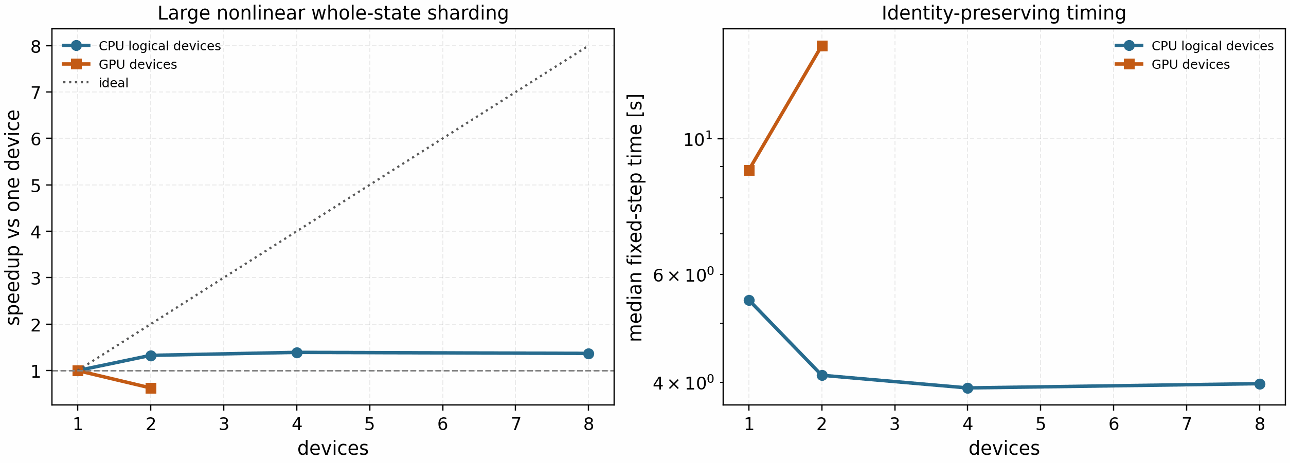
The refreshed large sweep remains engineering evidence rather than a speedup claim: it passed the final-state identity gate at every tracked point, the CPU logical-device path saturated at about 1.39x, and the June 21, 2026 two-RTX-A4000 auto route was slower than one GPU for the larger Nx=48, Ny=96, Nz=128, Nl=4, Nm=8 fixed-step case, with a measured strong scaling speedup of 0.586x. Current JAX/XLA CPU refreshes are stricter: unsafe active multi-device CPU whole-state pjit routes are skipped before execution and record a fail-closed blocker instead of producing a speedup row. This makes the technical conclusion explicit: whole-state nonlinear sharding is useful as a correctness/profiler gate, but production parallelization should prioritize independent k_y scans and UQ/ensemble batching. Communication-aware nonlinear domain decomposition remains diagnostic until the exact workload has identity, communication, transport-window, and matched profiler evidence for any nonlinear multi-GPU speedup claim. The production gate fails closed as diagnostic_only unless the refreshed CPU and GPU rows both pass serial identity, use active state sharding, and meet the configured speedup and parallel-efficiency thresholds. The tracked gate artifact is docs/_static/nonlinear_sharding_production_speedup_gate.json. In the current artifact set the CPU candidate is diagnostic and the refreshed GPU row is identity-complete but blocks production speedup claims because the speedup and efficiency gates fail. Its backend_blocker_report separates identity-evidence completeness from speedup/efficiency blockers, so an identity-correct slowdown is recorded as a useful negative result rather than as a promoted parallelization mode. The raw sweep JSON files also carry speedup_passed, status, and speedup_blockers fields so a timeout, profiler failure, or identity-correct slowdown is visible before the stricter production gate is evaluated.

This claim boundary is mirrored in Parallelization policy and Release Scope and Claim Boundaries. If a future optimization changes the conclusion, refresh the CPU and GPU sweep artifacts before changing README or release-note wording.

Spectral nonlinear mode (gated fast toggle)

The spectral nonlinear mode skips Laguerre quadrature for the nonlinear bracket (laguerre_nonlinear_mode = "spectral" or "fast"). It is not the default mode because the speedup is case and backend dependent. The release gate runs the same bounded nonlinear case twice, once with default grid-mode brackets and once with spectral brackets, then compares end-of-run scalar diagnostics.

python tools/artifacts/gate_laguerre_nonlinear_modes.py \
  --case cyclone --case kbm --case w7x --case hsx \
  --out-json docs/_static/laguerre_mode_gate.json \
  --out-csv docs/_static/laguerre_mode_gate.csv \
  --plot-out docs/_static/laguerre_mode_gate.png

For a GPU reference artifact, run the same command on the target GPU node with GPU-specific output paths, for example:

python tools/artifacts/gate_laguerre_nonlinear_modes.py \
  --case cyclone --case kbm --case w7x --case hsx \
  --out-json docs/_static/laguerre_mode_gate_gpu.json \
  --out-csv docs/_static/laguerre_mode_gate_gpu.csv \
  --plot-out docs/_static/laguerre_mode_gate_gpu.png

For W7-X/HSX runs, pass --w7x-geometry-file and --hsx-geometry-file if the local pre-generated *.eik.nc files live outside the default cache paths.

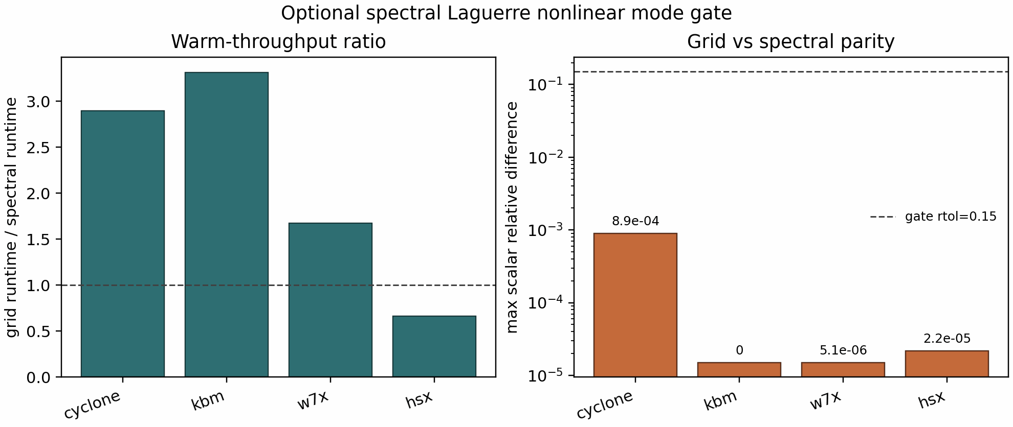
On the bounded local CPU gate, Cyclone, KBM, W7-X, and HSX all passed the scalar-diagnostic parity threshold with maximum relative differences below 8.9e-4. The measured grid/spectral runtime ratios were:

• Cyclone: 2.90

• KBM: 3.31

• W7-X: 1.67

• HSX: 0.66

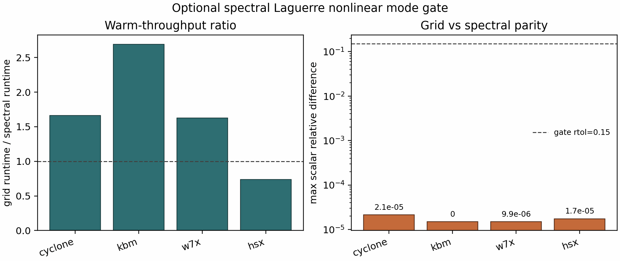
On the bounded office GPU gate, all four cases also passed with maximum relative differences below 2.2e-5. The measured grid/spectral runtime ratios were:

• Cyclone: 1.66

• KBM: 2.69

• W7-X: 1.63

• HSX: 0.74

Because HSX is slower in both bounded gates, the spectral mode should be treated as a validated optional engineering mode, not a global fast default.

A July 10, 2026 follow-up extended the Cyclone A4000 comparison from two steps to 400 steps (t=20) with a stricter five-percent gate. The spectral route passed with 8.71e-4 maximum relative scalar difference, 1.78e-4 heat-flux endpoint difference, and a 1.73x end-to-end runtime ratio. A matched kernel split measured grid-mode nonlinear_bracket=1.91e-2 s and full_rhs=2.74e-2 s versus spectral-mode 4.59e-3 s and 1.35e-2 s. This strengthens the bounded Cyclone fast-toggle evidence but does not replace the required long saturated-window gates for W7-X, HSX, and KBM.

The same refresh measured prepared 20-step wall times of 4.55 s on the local CPU (JAX 0.9.2) and 1.46 s on one office A4000 (JAX 0.4.38). Because those software stacks are not matched, these values are diagnostic and do not replace the README runtime panel or support a new CPU/GPU speedup claim. Production use should rerun the gate on the target case and backend before claiming speedup.

Runtime and memory comparison workflow

For the publication runtime comparison pass, use the manifest-driven runner:

python benchmarks/performance/benchmark_runtime_memory.py --list
python benchmarks/performance/benchmark_runtime_memory.py --dry-run --case cyclone-linear --backend gkx_cpu
python benchmarks/performance/benchmark_runtime_memory.py --continue-on-error --log-dir tools_out/runtime_memory_logs

The runner reads tools/runtime_memory_manifest.toml and writes:

• tools_out/runtime_memory_results.csv

• tools_out/runtime_memory_summary.json

• tools_out/runtime_memory_logs/*.stdout.log

• tools_out/runtime_memory_logs/*.stderr.log

• docs/_static/runtime_memory_benchmark.png

The promoted runtime/memory result files are also indexed from the root-level benchmarks/results/manifest.toml so users can find benchmark outputs without searching through scratch directories. Raw logs and NetCDF files should stay in tools_out/ or another scratch location; only the reviewed summary CSV/JSON and compressed panel are tracked.

The manifest is designed to hold three rows per case:

• gkx_cpu

• gkx_gpu

• gx

Each row may also carry a host so the same runner can execute local and remote measurements through one manifest while still collecting wall time and peak RSS from the target machine. Rows may also carry a profile_command. When that secondary command succeeds and prints warmup_time_s=... / run_time_s=..., the runner merges those warm measurements back into the same CSV/JSON summary row as the cold pass. If a profiling command prints warmup_time_s=... or run_time_s=..., the runner also records those fields in the CSV/JSON summary so cold and warm JAX timings can be tracked without a separate sidecar note.

The checked-in case inventory for the current release panel covers the shipped runtime families:

• Cyclone ITG linear and nonlinear

• ETG linear

• KBM linear and nonlinear

• W7-X linear and nonlinear

• HSX linear and nonlinear

• Cyclone Miller nonlinear

These rows are the ones shown in the README/runtime panel. ETG nonlinear, KAW, and TEM remain separate tracked work items and are intentionally excluded from the shipped runtime figure until their release-grade benchmark contracts are closed.

For the stellarator rows on the office benchmark host, the shipped panel uses pre-generated *.eik.nc geometry files instead of live VMEC regeneration. The GX reference rows on that host also need a consistent local netcdf-c / hdf5 runtime stack; the default office stellarator runtime environment mixed incompatible HDF5 / NetCDF libraries and lacked the Python geometry helper dependencies needed for VMEC-driven geometry generation.

Final runtime/memory figure

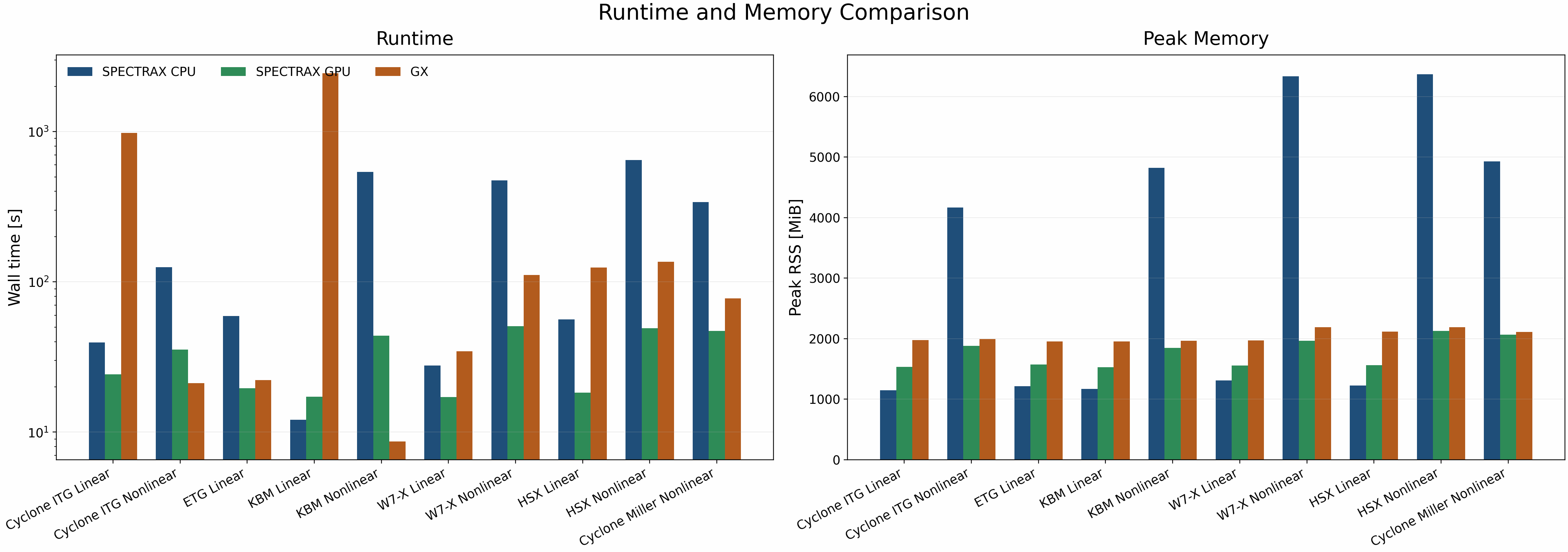
The runtime subplot uses a log scale because the measured wall times span roughly three orders of magnitude across the linear, nonlinear, and imported geometry cases. The memory subplot stays linear because the peak RSS spread is much narrower.

The assembled figure is generated from the collected per-case summaries with benchmarks/performance/benchmark_runtime_memory.py --summary-glob ... and written to:

• docs/_static/runtime_memory_benchmark.png

• docs/_static/runtime_memory_benchmark.pdf

For the shipped refresh shown here, use the successful release summary rather than the older interrupted summary that contains failed W7-X/HSX nonlinear rows:

python benchmarks/performance/benchmark_runtime_memory.py \
  --summary-glob docs/_static/runtime_memory_summary_ship_refresh.json \
  --csv-out docs/_static/runtime_memory_results_ship_refresh.csv \
  --summary-out docs/_static/runtime_memory_summary_ship_refresh.json \
  --plot-out docs/_static/runtime_memory_benchmark.png

The published runtime figure complements the atlas instead of duplicating it: the atlas carries growth/frequency and nonlinear transport/energy comparisons, while the runtime figure carries CPU/GPU/reference wall time and peak RSS for the shipped runtime cases.

Interpretation of short nonlinear GPU rows

The shipped runtime panel reports cold wall time. For the JAX backends, this includes startup and compilation, so short nonlinear cases can look worse than their steady-state throughput would suggest.

Targeted office GPU profiles on the same shipped short nonlinear configs measured:

Cyclone nonlinear: warmup_time_s=33.957  run_time_s=15.054
KBM nonlinear:     warmup_time_s=27.485  run_time_s= 9.725

Compared with the cold runtime panel rows:

• Cyclone nonlinear GPU: 38.27 s in the shipped panel, versus 15.05 s for the second run on the same compiled executable.

• KBM nonlinear GPU: 44.33 s in the shipped panel, versus 9.73 s for the second run on the same compiled executable.

This changes the optimization reading:

• the current short-run Cyclone GPU deficit in the shipped panel is primarily a cold-start effect, since the warm run is already faster than the tracked GX row,

• the current short-run KBM GPU gap is mostly compile amortization, with warm performance already close to GX.

The runtime figure now overlays those warm second-run measurements as hollow diamond markers on the runtime bars wherever run_time_s is present in the summary input.

The highest-value performance work for these short nonlinear lanes is therefore compile/startup reduction and executable reuse, not just per-step kernel work.

Startup phase profiler

For cold-start deep dives, use the dedicated startup profiler:

python tools/profiling/profile_startup_and_cache.py runtime-startup \
  --config examples/nonlinear/axisymmetric/runtime_cyclone_nonlinear.toml \
  --ky 0.3 --Nl 4 --Nm 8 --compile-steps 1 \
  --json-out tools_out/startup_cyclone_gpu.json \
  --csv-out tools_out/startup_cyclone_gpu.csv

The profiler breaks the cold path into the main setup and first-compile phases:

• runtime config load

• geometry resolution

• grid/default construction

• parameter and term setup

• initial-condition construction

• linear-cache construction

• first field solve compile+execute

• first linear/full RHS compile+execute

• first nonlinear integrator compile+execute

It supports --trace-dir and --memory-profile for XProf/Perfetto inspection with phase-level annotations, and --debug-log-cache / --explain-cache-misses for JAX cache diagnostics when a repeated compile path looks suspicious. By default the trace tools now start JAX profiling with python_tracer_level=0 and host_tracer_level=0. On the lightweight office environment this avoids the optional TensorFlow Python-hook import path, so traces are emitted cleanly without installing TensorFlow just to silence profiler startup noise.

The current office GPU startup profiles for the shipped short nonlinear cases show the same dominant structure:

• Cyclone nonlinear startup total: 35-36 s after the low-rank collision-cache and host-cache cleanup passes (previously 41.47 s on the earlier office snapshot)

• KBM nonlinear startup total: 32.23 s

• dominant phases in both cases:

  • compile_first_integrator_run: about 22 s (Cyclone), 19.28 s (KBM)

  • build_linear_cache: about 5.6 s (Cyclone), 7.73 s (KBM)

  • compile_first_linear_rhs / compile_first_full_rhs: another 3.0 + 3.0 s (Cyclone) or 1.7 + 1.7 s (KBM)

So the next high-value performance work is no longer the analytic geometry startup path or the collision prefactor path; it is the first compiled nonlinear integrator path, followed by the remaining Laguerre and drift/cache construction subphases.

To break the cache-construction lump down further, use:

python tools/profiling/profile_startup_and_cache.py linear-cache \
  --config examples/nonlinear/axisymmetric/runtime_cyclone_nonlinear.toml \
  --Nl 4 --Nm 8 \
  --json-out tools_out/linear_cache_cyclone_gpu.json \
  --csv-out tools_out/linear_cache_cyclone_gpu.csv

The current office GPU decomposition for the shipped Cyclone short nonlinear lane is:

• total measured decomposition: 6.86 s after the low-rank collision-cache, host-cache, and broadcasted-gyroaverage passes

• dominant subphases:

  • gyro_bessel_cache: 1.33 s

  • laguerre_cache: 1.21 s

  • kperp_and_drifts: 0.99 s

  • geometry_coefficients: 0.68 s

  • collision_and_damping_cache: 0.17 s

The low-rank collision cache, host-built moment/damping factors, and broadcasted gyroaverage construction remove the old collision/damping bottleneck from the cache profile. The overall cold-start wall clock is still dominated by the first nonlinear integrator compile. The next cache-build optimization work should therefore focus on Laguerre and drift/cache construction, while the broader startup campaign should prioritize the first integrator compile surface.

Cached basis indices

To reduce per-step overhead, the linear cache now stores Laguerre/Hermite index arrays (\(l\), \(m\)) and derived coefficients (l+1, m+1, sqrt(m), sqrt(m+1)). These are reused inside the mirror/curvature terms and the implicit preconditioner instead of re-allocating on every RHS call. The change is small in absolute cost for low-order runs, but becomes noticeable in higher-order scans and tight profiling loops.

GMRES preconditioner policy

The implicit linear solver exposes several preconditioner policies, with shape, finite-value, linked-boundary, and shift-invert contracts covered by the solver test suite rather than by an untracked ad-hoc profiling harness:

• diag: full diagonal (damping + drift + mirror)

• pas: PAS line preconditioner (streaming + diagonal damping/drifts)

• pas-coarse: line + kx-coarse additive correction (Schur-style)

• hermite-line: Hermite streaming line solve (tridiagonal in m at fixed \(k_z\))

• hermite-line-coarse: Hermite line solve + kx-coarse correction

Use tests/unit/linear/test_linear.py and tests/unit/linear/test_linear_helpers_extra.py as the maintained verification owners for these policies. Fresh runtime or iteration-count claims should be added through the tracked performance manifest and profiling tools, not through standalone probe scripts.

JIT considerations

The linear integrator is jit-compiled with the number of steps and method as static arguments. The operator term switches (gkx.operators.linear.params.LinearTerms) should also remain static inside a compiled loop to avoid recompilation. The cached operator arrays can be constructed once and reused across multiple runs to avoid repeated geometry setup costs. Nonlinear IMEX paths now reuse the electrostatic compiled linear-RHS route whenever apar=bpar=0; this is a bounded fast path for adiabatic-electron electrostatic runs, not a new runtime claim until a fresh end-to-end profile is recorded.

Planned optimizations

• vmap over species and parameter scans

• JAX mesh-based parallelization across multiple devices

• FFT acceleration and layout tuning

• operator fusion for nonlinear terms

Linear-to-nonlinear optimization roadmap

The current benchmark runtime gap on CPU is dominated by JAX compile latency and repeated small-shape scan launches. The next implementation phase targets both linear and nonlinear performance with a single operator strategy:

1. Compile-once scan kernels

   • enforce fixed batch shapes across ky and beta scans,

   • pre-JIT a small set of canonical (Nl, Nm, Ny, Nz) signatures,

   • cache compiled executables on disk for repeated benchmark sweeps.

2. Operator fusion in RHS assembly

   • merge streaming/mirror/curvature/grad-B stencils into one fused kernel,

   • remove scatter-heavy intermediate writes,

   • keep field coupling and species sums contiguous in memory.

3. Matrix-free eigen path as default for linear scans

   • use Krylov/shift-invert for scan tables and figures,

   • reserve long time integration for spot-check diagnostics only.

4. Preconditioner reuse

   • persist Hermite-line and shift-invert preconditioner structures across neighboring scan points (same geometry/grid),

   • reuse Jacobian-like linearization objects in IMEX stages.

5. Streaming diagnostics by default

   • avoid storing full time traces unless explicitly requested,

   • compute growth/frequency online from selected mode signals.

These steps are chosen to carry directly into nonlinear runs, where the same fused RHS, scan batching, and preconditioner reuse will dominate throughput and memory behavior.