Examples

The examples directory is organized around two layers:

• case-backed runtime drivers that map directly onto the tracked runtime TOMLs,

• focused demos and benchmark helpers for theory, operators, and scan workflows.

Config-backed runtime cases

These scripts are the closest match to the production benchmark workflows. They load the checked-in runtime TOMLs and expose only the most useful runtime overrides at the command line.

Tokamak cases

python examples/linear/axisymmetric/cyclone_runtime_linear.py
python examples/nonlinear/axisymmetric/cyclone_runtime_nonlinear.py --steps 200
python examples/nonlinear/axisymmetric/cetg_runtime_nonlinear.py --steps 1000
python examples/linear/axisymmetric/etg_runtime_linear.py
python examples/linear/axisymmetric/kaw_runtime_linear.py
python examples/linear/axisymmetric/kbm_runtime_linear.py
python examples/nonlinear/axisymmetric/kbm_runtime_nonlinear.py --steps 200
python examples/nonlinear/axisymmetric/miller_nonlinear_runtime.py --steps 200

Stellarator and imported-geometry cases

python examples/linear/non-axisymmetric/w7x_linear_imported_geometry.py \
  --geometry-file /path/to/itg_w7x_adiabatic_electrons.eik.nc

python examples/linear/non-axisymmetric/hsx_linear_imported_geometry.py \
  --geometry-file /path/to/hsx_linear.eik.nc

python examples/nonlinear/non-axisymmetric/w7x_nonlinear_imported_geometry.py \
  --geometry-file /path/to/w7x_adiabatic_electrons.eik.nc

python examples/nonlinear/non-axisymmetric/hsx_nonlinear_imported_geometry.py \
  --geometry-file /path/to/hsx_nonlinear.eik.nc

export W7X_VMEC_FILE=/absolute/path/to/wout_w7x.nc
export HSX_VMEC_FILE=/absolute/path/to/wout_HSX_QHS_vac.nc
python examples/nonlinear/non-axisymmetric/w7x_nonlinear_vmec_geometry.py --steps 200
python examples/nonlinear/non-axisymmetric/hsx_nonlinear_vmec_geometry.py --steps 200

For the VMEC-backed stellarator examples, omit --steps when you want the default adaptive horizon. Set --steps only when you intentionally want a short profiling or diagnostic window. For longer W7-X nonlinear runs, keep adaptive timesteps enabled (the default for the examples) or reduce dt if you need a fixed-step stability study.

The shipped nonlinear stellarator runtime TOMLs now also emit artifact bundles under tools_out/ by default:

• tools_out/w7x_nonlinear_vmec_runtime.diagnostics.csv

• tools_out/hsx_nonlinear_vmec_runtime.diagnostics.csv

• tools_out/w7x_nonlinear_imported_runtime.diagnostics.csv

Those diagnostics and their matching *.summary.json files are the intended inputs for the parity helpers under tools/. The direct Python runtime wrappers now route through the same artifact-aware nonlinear path as the executable, so long adaptive runs update that bundle as each chunk completes.

Runtime TOML entry points

When you want the full config surface instead of the thin case wrappers, use the executable or the generic example drivers directly. These runtime utilities are best treated as solver-smoke and exploration entry points; the benchmark examples remain the audited parity surface for ETG and the other validation lanes:

python examples/utilities/runtime_from_toml.py --config examples/linear/axisymmetric/runtime_cyclone.toml
python examples/utilities/runtime_from_toml.py --config examples/linear/axisymmetric/runtime_etg.toml
python examples/utilities/runtime_from_toml.py --config examples/linear/axisymmetric/runtime_kbm.toml
python examples/linear/axisymmetric/etg_linear_auto.py --outdir tools_out/etg_auto

spectrax-gk run-runtime-linear \
  --config examples/linear/axisymmetric/runtime_cyclone_quasilinear.toml \
  --out tools_out/cyclone_quasilinear

spectrax-gk run-runtime-linear \
  --config examples/linear/non-axisymmetric/runtime_w7x_linear_imported_geometry.toml

spectrax-gk examples/linear/axisymmetric/runtime_cyclone.toml

For a bounded runtime-configured independent k_y scan that uses [parallel] strategy = "batch" without changing the single-k_y solver layout, run:

python examples/parallelization/independent_ky_runtime_batch_scan.py

The companion examples/parallelization/runtime_batch_ky_scan.toml selects two thread workers through [parallel].num_devices. The runtime still dispatches normal single-k_y solver calls and gathers results in input order; it does not opt into the combined-k_y solver path.

Scaling utilities

For production parallelization of independent scans and UQ ensembles, prefer the package helpers:

import jax.numpy as jnp
import spectraxgk as sgk

ky = jnp.asarray([0.1, 0.2, 0.3, 0.4])
chunks = sgk.ky_scan_batches(ky, n_batches=2)
values = sgk.batch_map(
    lambda x: {"gamma": x, "ql_weight": x**2},
    ky,
    batch_size=2,
)

For file-backed calibration and uncertainty workflows that are independent but not JAX-array vmap workloads, use sgk.independent_map:

rows = sgk.independent_map(
    lambda case: {"case": case, "score": len(case)},
    ["cyclone", "hsx", "w7x"],
    workers=2,
)

These helpers preserve serial ordering and fall back to a one-device vmap path on laptops. Multi-device runs should still be checked against the serial result before publication speedups are claimed.

Autodiff validation reports also accept workers for thread-parallel central finite-difference columns, and the stellarator optimization comparison script exposes the same pattern:

JAX_ENABLE_X64=1 python examples/optimization/compare_stellarator_itg_optimizations.py \
  --workers 3 \
  --finite-difference-workers 2

The generated JSON records both worker counts and keeps the acceptance criterion as numerical identity with the serial report.

For a solver-backed identity gate, run the Cyclone k_y-batch scan artifact:

python tools/generate_parallel_ky_scan_gate.py

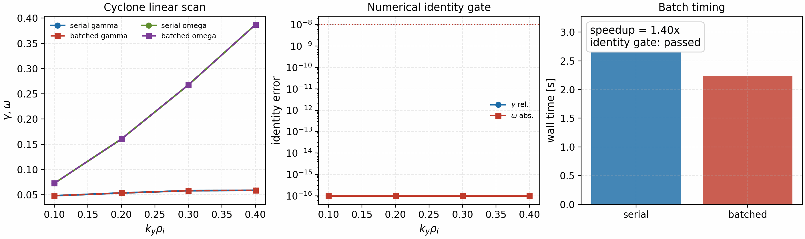
Real Cyclone linear solver comparison between serial and fixed-shape k_y-batched scans. The figure verifies that gamma and omega are identical while reporting the observed batch speedup separately.

For a logical-CPU API gate that exercises RuntimeParallelConfig and pytree outputs, run:

python tools/generate_logical_cpu_parallel_scan_gate.py --logical-devices 2

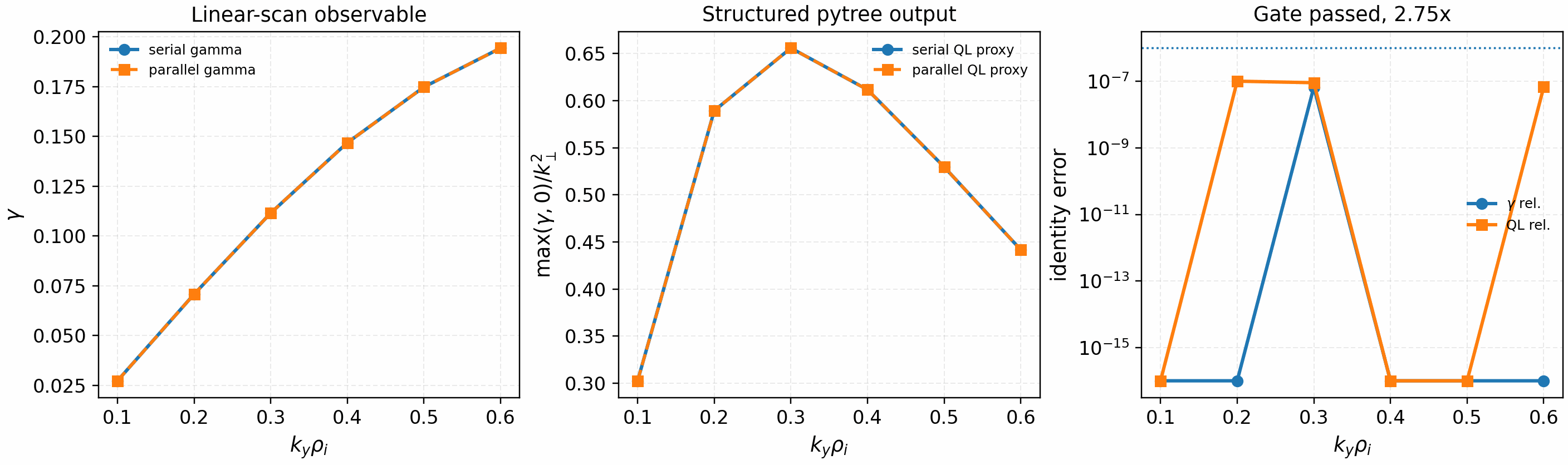
Independent-scan interface gate for structured outputs. This validates the parallel API used by UQ and sensitivity ensembles; it is not a nonlinear performance claim.

The first lower-level communication gate for velocity-space decomposition is the Hermite ghost exchange:

python tools/generate_hermite_exchange_gate.py --logical-devices 2

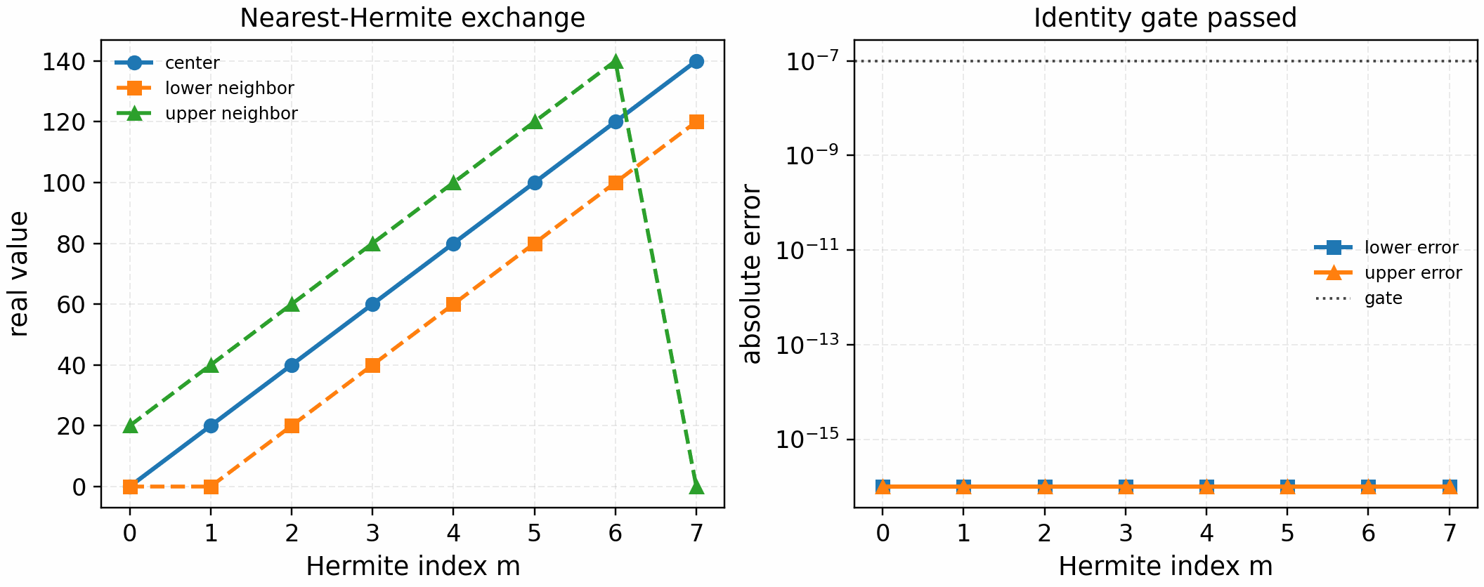
shard_map nearest-neighbor exchange for Hermite moments. This validates the communication primitive that a future nonlinear velocity-space sharding path needs before field reductions and full-RHS identity gates are added.

The paired field-reduction gate is:

python tools/generate_velocity_field_reduce_gate.py --logical-devices 2

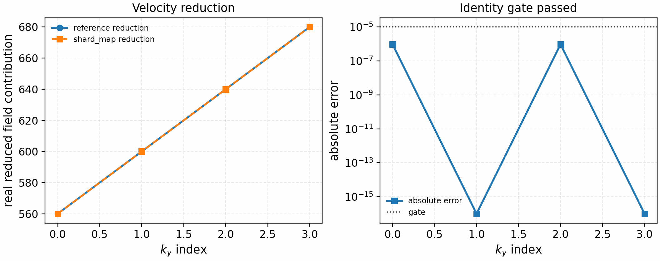
shard_map reduction/broadcast over a Hermite mesh. This establishes the field-solve communication primitive before streaming-ladder and nonlinear RHS identity gates are attempted.

The first production-field-solve reduction gate is:

python tools/generate_electrostatic_field_reduce_gate.py --logical-devices 2

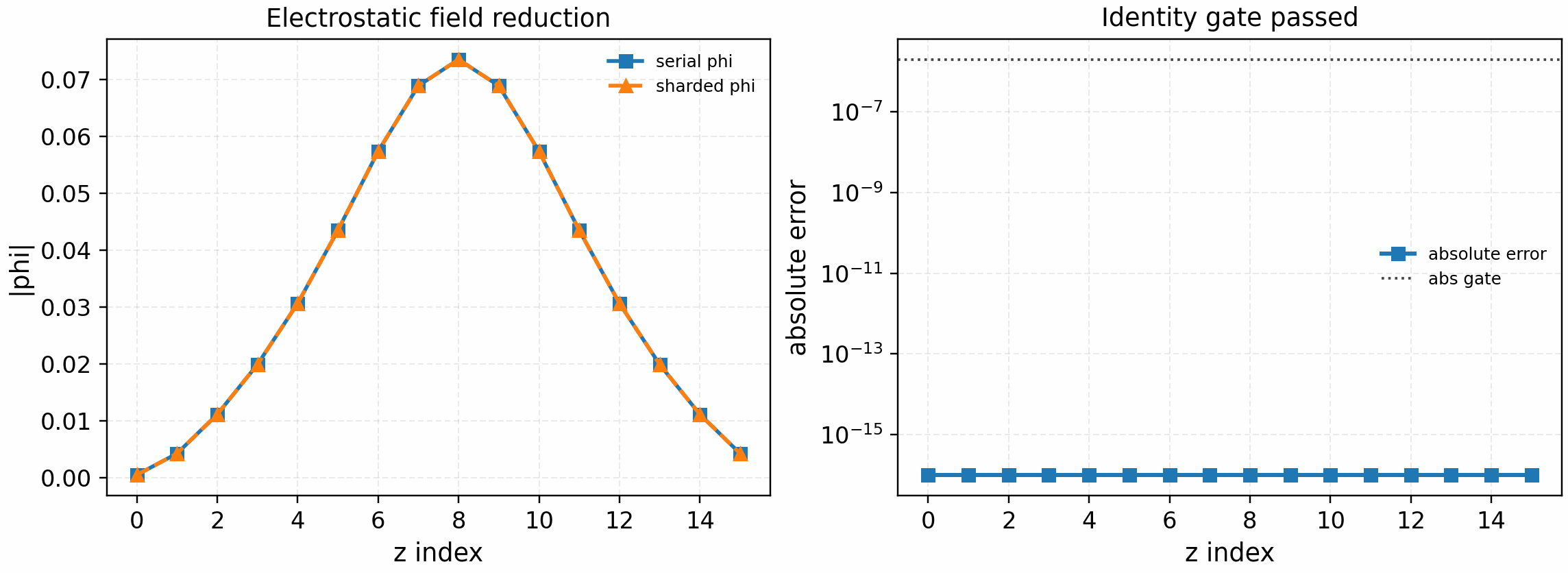
Hermite-sharded m=0 density reduction for the electrostatic quasineutrality solve, compared against the production field solve.

The Hermite streaming-ladder coefficient gate is:

python tools/generate_hermite_streaming_ladder_gate.py --logical-devices 2

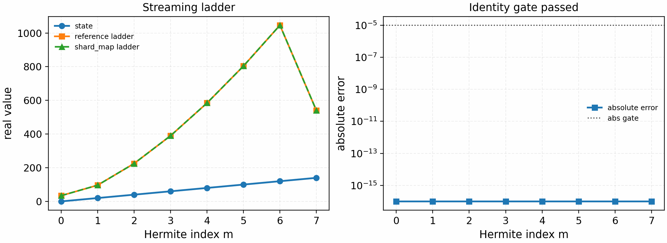
shard_map Hermite exchange plus the sqrt(m+1) / sqrt(m) streaming-ladder coefficients. This is still a communication/coefficient gate; full linear streaming also needs the parallel derivative identity gate before production runtime wiring.

The first electrostatic drift-slice gate is:

python tools/generate_electrostatic_drift_gate.py --logical-devices 2

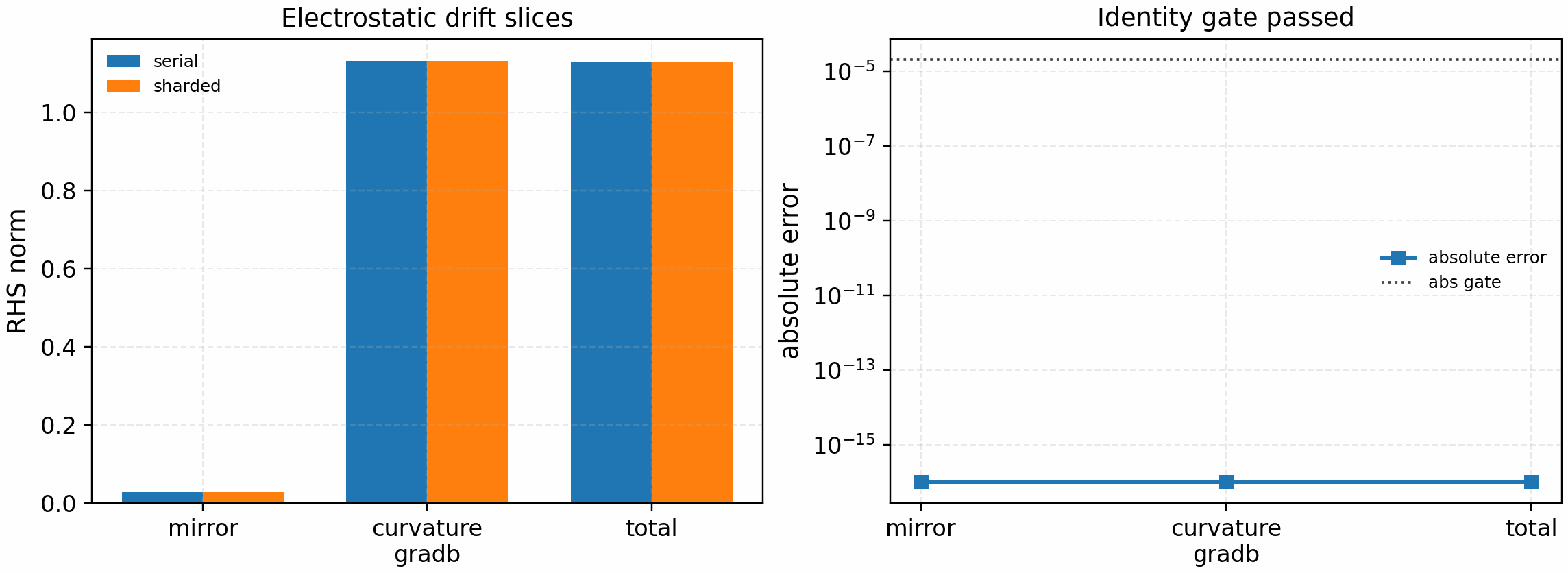
Hermite-sharded mirror and curvature/grad-B drift slices, including offset-1 and offset-2 Hermite exchanges, compared against the production linear RHS with only those terms enabled.

The matching electrostatic diamagnetic-drive gate is:

python tools/generate_electrostatic_diamagnetic_gate.py --logical-devices 2

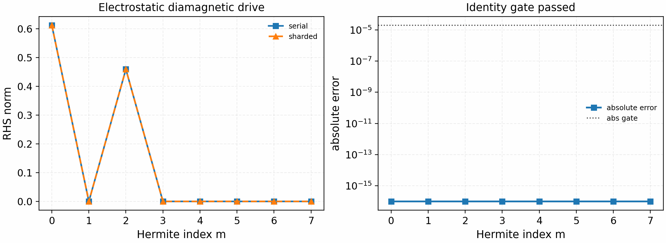
Hermite-sharded electrostatic diamagnetic drive. The sharded route first uses the electrostatic field-reduction gate, then applies the local m=0 and m=2 drive masks on each Hermite shard. This closes the diamagnetic slice for the opt-in electrostatic linear-slices backend.

The periodic streaming microkernel gate adds that field-line derivative:

python tools/generate_periodic_streaming_microkernel_gate.py --logical-devices 2

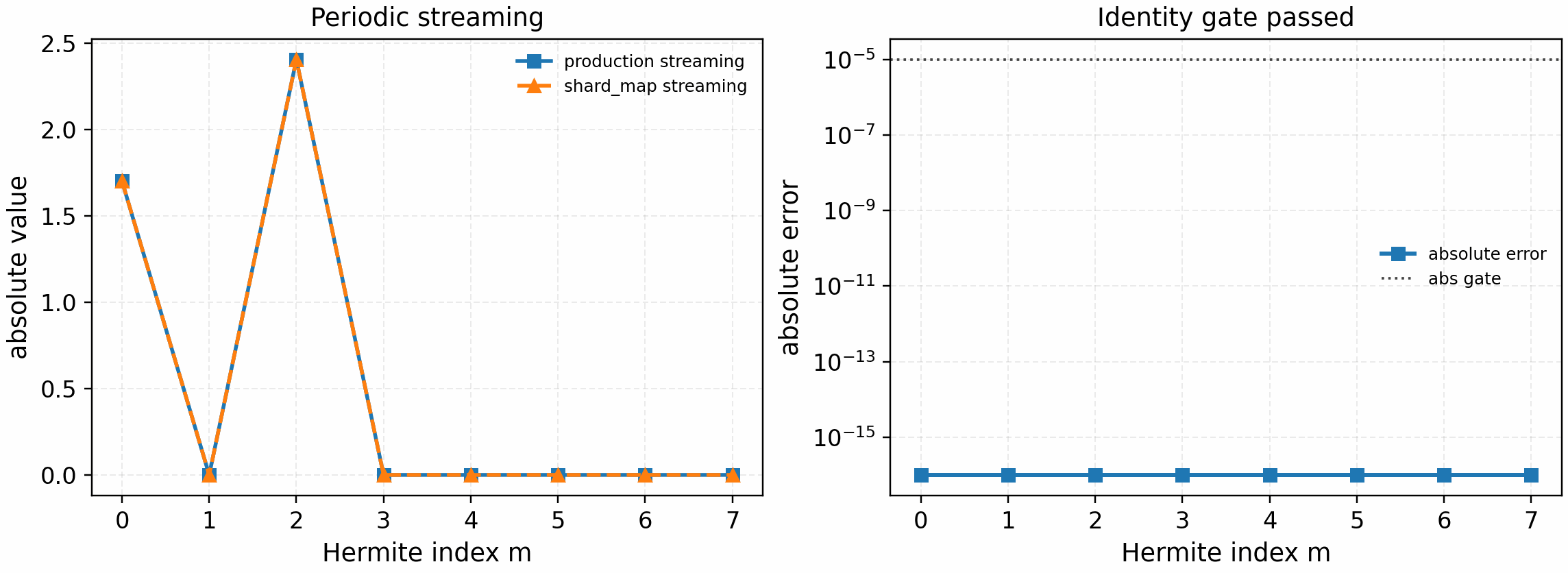
Periodic spectral parallel derivative plus Hermite streaming ladder through the shard_map path, compared directly against the production streaming operator.

The next gate places that same sharded streaming kernel under the production linear-RHS call graph with every non-streaming contribution disabled:

python tools/generate_linear_rhs_streaming_gate.py --logical-devices 2

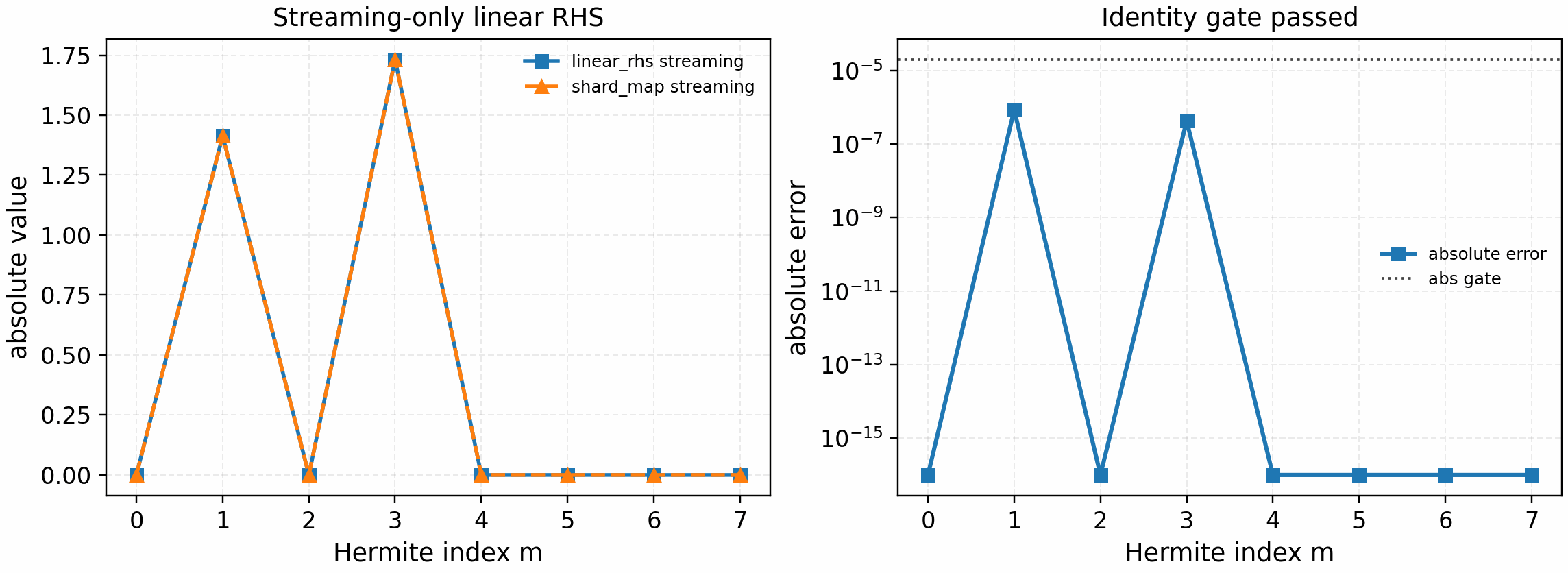
Streaming-only linear_rhs_cached comparison against the velocity-sharded periodic streaming path. This closes the first full-RHS call-graph identity gate for the streaming term only; it is not yet a full linear scan or nonlinear speedup claim.

With a nonzero electrostatic response, use:

python tools/generate_linear_rhs_streaming_electrostatic_gate.py --logical-devices 2

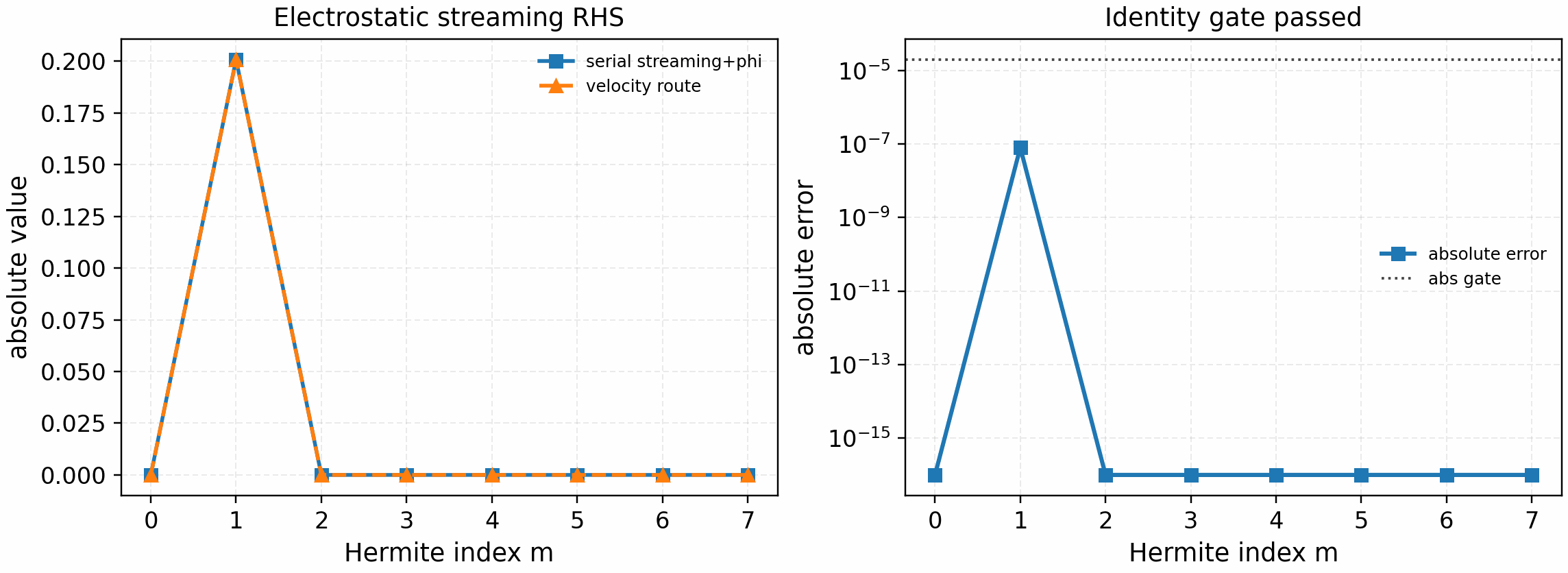
Streaming plus electrostatic phi call-graph comparison. The field solve uses the Hermite-sharded electrostatic reduction gate; this validates the next velocity-sharded streaming slice before drift, diamagnetic-drive, and nonlinear terms are introduced.

For the composed electrostatic linear-slices backend, use:

python tools/generate_linear_rhs_electrostatic_slices_gate.py --logical-devices 2

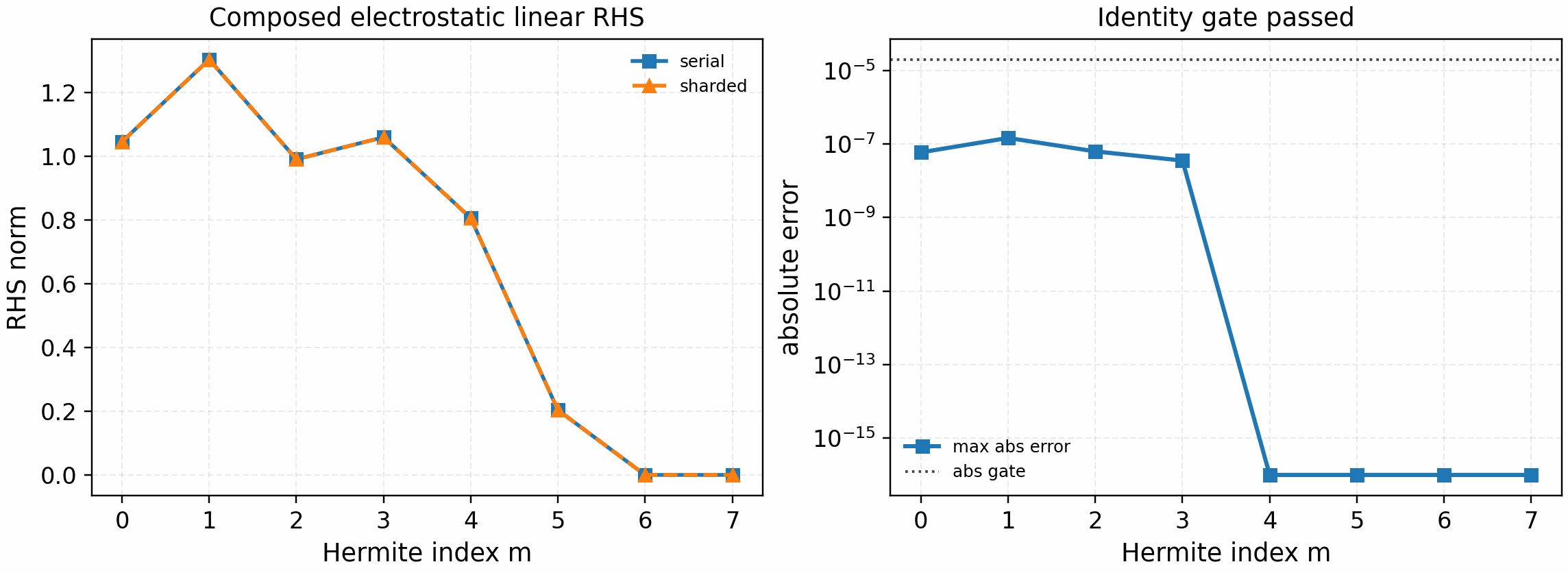
Full opt-in electrostatic linear-slices call-graph comparison for streaming, mirror, curvature, grad-B, and diamagnetic drive. This is the current production-parallelization identity artifact for the single-species periodic electrostatic RHS path; collisions, linked boundaries, electromagnetic terms, and nonlinear brackets remain separate gates.

Use the strong-scaling sweep helper to collect parallelization timings for the distributed linear RK2 loop:

python examples/utilities/strong_scaling_sweep.py \
  --ny 128 --nz 256 --nl 8 --nm 8 --steps 120 \
  --devices 1,2,4,8 \
  --backend cpu_parallel_large \
  --out tools_out/strong_scaling_cpu.csv

On multi-GPU systems, point --devices at the available accelerators and update --backend accordingly (for example cuda_parallel_large). The backend labels are just sweep names for the output table; they do not change the runtime physics or solver path.

For the current opt-in Hermite-sharded electrostatic linear RHS path, use the engineering sweep helper:

python tools/profile_linear_rhs_parallel_slices_sweep.py \
  --platform cpu --devices 1,2,4,8 --nms 64,128 \
  --nl 4 --ny 32 --nz 128 --rtol 1e-5

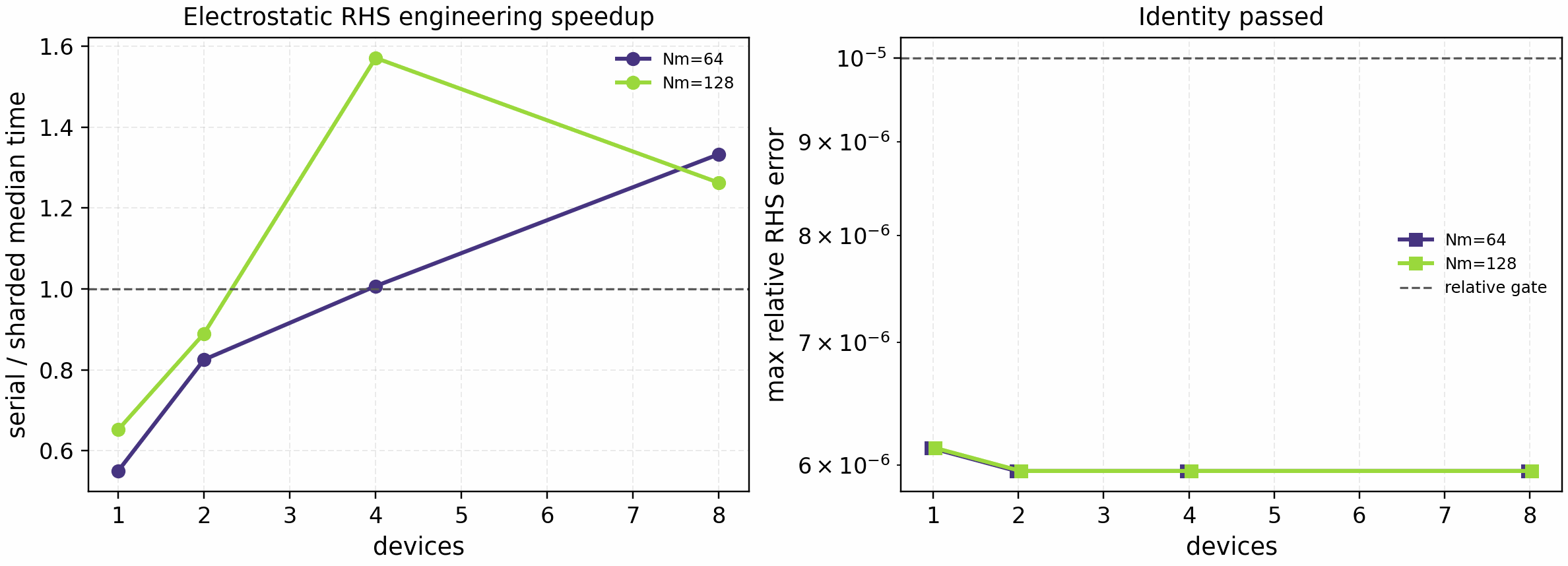
Device-count and Hermite-resolution sweep for the opt-in electrostatic linear-slices backend. The right panel is the identity gate; the left panel is engineering timing only and should not be promoted as a nonlinear or publication speedup claim.

Plotting outputs

To visualize nonlinear diagnostic histories from *.out.nc files:

python examples/utilities/plot_runtime_outputs.py tools_out/cyclone_release.out.nc \
  --out tools_out/cyclone_release_diagnostics.png

Geometry examples

VMEC and Miller geometry usage examples are documented in Geometry.

Nonlinear restart and continuation

The tracked nonlinear runtime path supports a NetCDF out/big/restart bundle together with continuation from the saved restart state.

One-shot nonlinear bundle write:

spectrax-gk run-runtime-nonlinear \
  --config examples/nonlinear/axisymmetric/runtime_cyclone_nonlinear.toml \
  --steps 200 \
  --out tools_out/cyclone_release.out.nc

For the short GX-reference Cyclone replay (t_max = 5, no collisions), use examples/nonlinear/axisymmetric/runtime_cyclone_nonlinear_short.toml. That file pins the short-run dissipation contract explicitly (p_hyper = 2, damp_ends_amp = 0) instead of relying on the longer production defaults.

Restart-aware TOML snippet:

[time]
nstep_restart = 100

[output]
path = "tools_out/cyclone_release.out.nc"
restart_if_exists = true
save_for_restart = true
append_on_restart = true
restart_with_perturb = false

With that configuration, rerunning the same nonlinear command resumes from tools_out/cyclone_release.restart.nc when it already exists and appends the continued history to tools_out/cyclone_release.out.nc. This is the recommended user-facing workflow for long nonlinear turbulence jobs.

Geometry helper workflows

The runtime geometry path can generate imported geometry files from VMEC and Miller inputs when the external helper scripts are available:

export W7X_VMEC_FILE=/absolute/path/to/wout_w7x.nc
export HSX_VMEC_FILE=/absolute/path/to/wout_HSX_QHS_vac.nc
export SPECTRAX_BOOZ_XFORM_JAX_PATH=/absolute/path/to/booz_xform_jax
python tools/generate_gx_vmec_eik.py \
  --config examples/nonlinear/non-axisymmetric/runtime_hsx_nonlinear_vmec_geometry.toml

python tools/generate_gx_miller_eik.py \
  --config examples/nonlinear/axisymmetric/runtime_cyclone_nonlinear_miller.toml

Benchmark and scan helpers

These scripts produce the scan-level plots and tables used in the benchmark discussion:

python examples/benchmarks/cyclone_linear_benchmark.py
python examples/linear/axisymmetric/etg_linear_auto.py
python examples/benchmarks/etg_linear_benchmark.py
python examples/benchmarks/kbm_beta_scan.py
python examples/benchmarks/kinetic_linear_benchmark.py
python examples/benchmarks/tem_linear_benchmark.py

Foundational demos

These smaller examples are useful for understanding the numerical building blocks without running a full benchmark case:

python examples/benchmarks/basis_orthonormality.py
python examples/theory_and_demos/cyclone_geometry.py
python examples/theory_and_demos/autodiff_inverse_growth.py
python examples/theory_and_demos/autodiff_inverse_twomode.py
python examples/theory_and_demos/diffrax_linear_demo.py
python examples/theory_and_demos/example.py
python examples/theory_and_demos/gradB_coupling_hl_1d.py
python examples/theory_and_demos/linear_rhs_demo.py
python examples/theory_and_demos/two_stream_hermite_1d.py

The autodiff demos write summary JSON plus R/L_Ti and R/L_n sweep CSVs in the chosen output directory alongside the publication-ready plots. The single-mode figure is a local inverse/sensitivity example; the two-mode figure is the release-grade parameter-recovery validation.

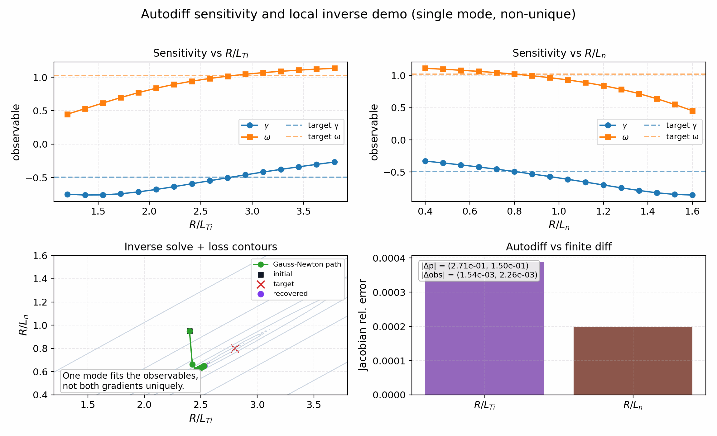
Single-mode inverse/sensitivity demo. The goal is to verify the autodiff Jacobian and show what one measured mode constrains locally; the expected outcome is small observable and derivative error, not unique recovery of both gradients. The shipped result matches that expectation: (gamma, omega) are reproduced closely while the recovered (R/L_Ti, R/L_n) remains offset because the one-mode inverse is not globally identifiable.

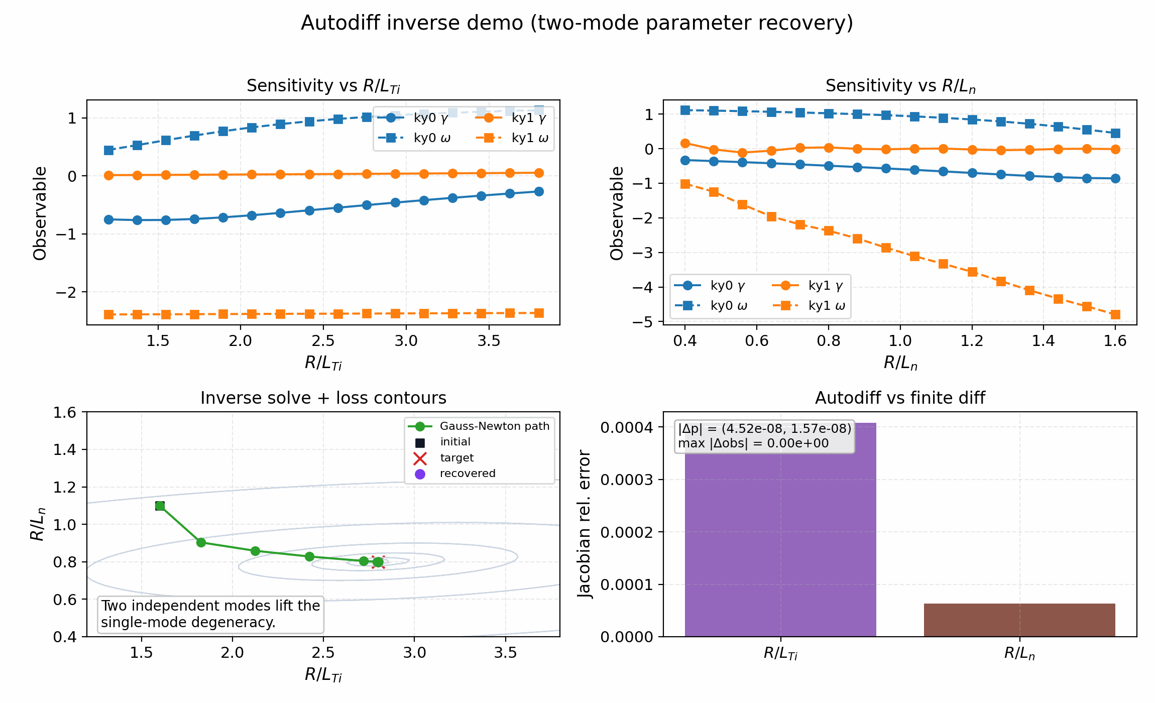
Two-mode inverse validation. The goal is to recover the planted gradients from two independent mode observables and verify that the autodiff Jacobian stays consistent with finite differences. The shipped result reaches the target to numerical precision and is the reviewer-facing parameter-recovery validation.

Secondary slab workflow

python -m spectraxgk.cli run-runtime-linear \
  --config examples/benchmarks/runtime_secondary_slab.toml

python examples/benchmarks/secondary_slab_workflow.py

The staged helper runs the linear seed, writes a restart state in the runtime binary layout, and then launches the nonlinear follow-up with the matching restart and fixed-mode controls used in the tracked secondary benchmark.

Reduced-model runtime

python examples/nonlinear/axisymmetric/cetg_runtime_nonlinear.py --steps 1000
spectrax-gk examples/nonlinear/axisymmetric/runtime_cetg_reference.toml --steps 1000

The reduced collisional slab ETG workflow uses the dedicated cETG runtime solver rather than the full-GK field solve path.

Full-GK ETG nonlinear pilot

python examples/nonlinear/axisymmetric/etg_runtime_nonlinear.py --steps 200
JAX_ENABLE_X64=1 spectrax-gk examples/nonlinear/axisymmetric/runtime_etg_nonlinear.toml --steps 200

This is the full-GK two-species ETG nonlinear pilot lane. It is intentionally separate from the reduced cETG workflow. The shipped contract now matches the audited GX short-window startup path: Lx = 1.25 for the linked ETG box and gaussian_init = true with init_single = false because GX reads init_single from its [Expert] section, not from [Initialization].